High-Accuracy Confidence Regions for Distribution Parameters

Jan Vrbik

Department of Mathematics and Statistics, Brock University, St. Catharines, Canada.

DOI: 10.4236/am.2022.136031                

Abstract

With the help of today’s computers, it is always relatively easy to find maximum-likelihood estimators of one or more parameters of any specific statistical distribution, and use these to construct the corresponding approximate confidence interval/region, facilitated by the well-known asymptotic properties of the likelihood function. The purpose of this article is to make this approximation substantially more accurate by extending the Taylor expansion of the corresponding probability density function to include quadratic and cubic terms in several centralized sample means, and thus finding the corresponding -proportional correction to the original algorithm. We then demonstrate the new procedure’s usage, both for constructing confidence regions and for testing hypotheses, emphasizing that incorporating this correction carries minimal computational and programming cost. In our final chapter, we present two examples to indicate how significantly the new approximation improves the procedure’s accuracy.

Keywords

High-Accuracy Confidence Regions, Distribution Parameters

1. Introduction

Using the likelihood function to find an approximate confidence region for several parameters (often only one, in which case we speak of a confidence interval) of a specific distribution goes back to the classic publication of Kendall and Stuart [1] . To understand the rest of our article, it is necessary to briefly review their main result, summarized by

Theorem 1. Assuming a case of regular (meaning the distribution’s support is not a function of any of the distribution’s parameters) estimation, the following random variable

$2\ln L\left(X\mathrm{<mo>\; ;\; </mo>}\hat{\theta }\right)-2\ln L\left(X\mathrm{<mo>\; ;\; </mo>}{\theta }_0\right)$ (1)

has approximately the chi-square distribution with K degrees of freedom, where K is the number of parameters to be estimated, $X$ is the set of n observations (allowing for the possibility of a multivariate distribution), $L\left(X\mathrm{<mo>\; ;\; </mo>}\theta \right)$ denotes the corresponding likelihood function, $\hat{\theta }$ is the vector of the resulting ML estimates, and ${\theta }_0$ represents the true (but unknown) values of the parameters.

Proof. Realizing that

$\ln L\left(X\mathrm{<mo>\; ;\; </mo>}\theta \right)\mathrm{<mo>\; :\; </mo>}={\displaystyle \underset{i=1}{\overset{n}{\sum }}}\ln f\left(x_i\mathrm{<mo>\; ;\; </mo>}\theta \right)$ (2)

where $x_i$ are the individual observations, then differentiating the RHS with respect to $\theta$ and setting each component of the answer to 0 yields

${\displaystyle \underset{i=1}{\overset{n}{\sum }}}\frac{\partial \ln f\left(x_i\mathrm{<mo>\; ;\; </mo>}\theta \right)}{\partial \theta }=0$ (3)

where $\frac{\partial }{\partial \theta }$ implies differentiating $\ln f\left(x_i\mathrm{<mo>\; ;\; </mo>}\theta \right)$ with respect to each parameter; the result is thus a vector with K components.

To solve the corresponding set of equations, we expand the LHS of (3) at $\theta ={\theta }_0$ , thus getting

${\displaystyle \underset{i=1}{\overset{n}{\sum }}}{\frac{\partial \ln f\left(x_i\mathrm{<mo>\; ;\; </mo>}\theta \right)}{\partial \theta }|}_{\theta ={\theta }_0}+{\displaystyle \underset{i=1}{\overset{n}{\sum }}}{\frac{{\partial }^2\ln f\left(x_i\mathrm{<mo>\; ;\; </mo>}\theta \right)}{\partial {\theta }^2}|}_{\theta ={\theta }_0}\left(\theta -{\theta }_0\right)+\cdots =0$ (4)

where the second derivative of $\ln f\left(x_i\mathrm{<mo>\; ;\; </mo>}\theta \right)$ is a symmetric K by K matrix. Dividing each side of the last equation by n, we solve it for $\theta -{\theta }_0$ getting, to the first-order accuracy

$\hat{\theta }-{\theta }_0\simeq -{\mu }_2^{-1}Y$ (5)

where

$Y\mathrm{<mo>\; :\; </mo>}=\frac{1}{n}{\displaystyle \underset{i=1}{\overset{n}{\sum }}}{\frac{\partial \ln f\left(x_i\mathrm{<mo>\; ;\; </mo>}\theta \right)}{\partial \theta }|}_{\theta ={\theta }_0}$ (6)

${\mu }_2\mathrm{<mo>\; :\; </mo>}=\mathbb{E}\left({\frac{{\partial }^2\ln f\left(X\mathrm{<mo>\; ;\; </mo>}\theta \right)}{\partial {\theta }^2}|}_{\theta ={\theta }_0}\right)$ (7)

Note that the expected value of $Y$ is $0$ , since

${\displaystyle {\int }_{\text{All}x}\frac{\partial \ln f\left(x\mathrm{<mo>\; ;\; </mo>}\theta \right)}{\partial \theta }f\left(x\mathrm{<mo>\; ;\; </mo>}\theta \right)\text{d}x}={\displaystyle {\int }_{\text{All}x}\frac{\partial f\left(x\mathrm{<mo>\; ;\; </mo>}\theta \right)}{\partial \theta }\text{d}x}=\frac{\partial }{\partial \theta }\left(1\right)=0$ (8)

and its variance-covariance matrix equals to $-{\mu }_2/n$ , due to

$\frac{\text{d}}{\text{d}\theta }{\displaystyle {\int }_{\text{All}x}\frac{\partial \ln f\left(x\mathrm{<mo>\; ;\; </mo>}\theta \right)}{\partial \theta }f\left(x\mathrm{<mo>\; ;\; </mo>}\theta \right)\text{d}x}={\mu }_2+{\mu }_{11}=\mathbb{O}$ (9)

where

${\mu }_{11}\mathrm{<mo>\; :\; </mo>}=\mathbb{E}\left({\frac{\partial \ln f\left(X\mathrm{<mo>\; ;\; </mo>}\theta \right)}{\partial \theta }\circ \frac{\partial \ln f\left(X\mathrm{<mo>\; ;\; </mo>}\theta \right)}{\partial \theta }|}_{\theta ={\theta }_0}\right)$ (10)

is the variance-covariance matrix of ${\frac{\partial \ln f\left(X\mathrm{<mo>\; ;\; </mo>}\theta \right)}{\partial \theta }|}_{\theta ={\theta }_0}$ (the small circle implies direct product of the two vectors), and $\mathbb{O}$ is the zero matrix.

Similarly expanding (1) and utilizing (5) we get, to the same level of accuracy

$2nY\left(\hat{\theta }-{\theta }_0\right)+n{\left(\hat{\theta }-{\theta }_0\right)}^{\text{T}}{\mu }_2\left(\hat{\theta }-{\theta }_0\right)=-n{Y}^{\text{T}}{\mu }_2^{-1}Y$ (11)

resulting in the following simple approximation to (1)

$-\sqrt{n}{Y}^{\text{T}}{\mu }_2^{-1}Y\sqrt{n}$ (12)

where $Y\sqrt{n}$ has (due to Central Limit Theorem) a K-variate Normal distribution with the mean of $0$ and the variance-covariance matrix of $-{\mu }_2$ . Introducing $Z=Y\sqrt{n}$ , the moment generating function of (12) is then computed by

$\begin{array}{l}\frac{{\displaystyle {\int }_{-\infty }^{\infty }\exp \left(-\frac{z^{\text{T}}{\left(-{\mu }_2\right)}^{-1}z}{2}+t{z}^{\text{T}}{\left(-{\mu }_2\right)}^{-1}z\right)\text{d}z}}{{\left(2\pi \right)}^{K/2}\sqrt{\det \left(-{\mu }_2\right)}}\\ =\sqrt{\det \left(\frac{-{\mu }_2}{1-2t}{\left(-{\mu }_2\right)}^{-1}\right)}={\left(1-2t\right)}^{-K/2}\end{array}$ (13)

easily identified as the MGF of ${\chi }_K^2$ distribution. ■

The result then leads to a simple (we call it basic) algorithm of constructing the corresponding confidence region based on a random independent sample of n observations.

Examples

From the last theorem it follows that an approximate confidence region is found by following these steps:

● Using sample values drawn from the distribution, maximize its likelihood function, thus getting the ML estimates of all parameters;

● Choose a confidence level (denoted $\tau$ ) and make (1) (where $\hat{\theta }$ represents the ML estimates, but ${\theta }_0$ are now variables to be solved for) equal to the corresponding critical value of the ${\chi }_K^2$ distribution;

● Solve for ${\theta }_0$ , resulting in two limits of the corresponding confidence interval when $K=1$ , a closed curve when $K=2$ , a closed surface when $K=3$ , etc.; this means that, beyond a one-parameter case, the resulting region can be displayed only graphically (a trivial task for today’s computers).

The following Mathematica program shows how it is done, first using a Geometric distribution with a (computer generated) sample of 40 and confidence level of 90%, then a Gamma distribution with a sample of 60 and confidence level of 95%.

The last line of the program has produced the following 95% confidence region (see Figure 1) for α (horizontal scale) and β (vertical scale).

A three-parameter estimation can be done in a similar manner, only the call to “ContourPlot” needs to be replaced by “ContourPlot3D”. Visualizing a confidence region for more than three parameters would require slicing it into a sequence of cross-sections.

Figure 1. Confidence region for α and β.

The error of this procedure depends on the sample size, decreasing with n in the $O\left(\frac{1}{n}\right)$ manner; it can reach several percent for small samples. The purpose of the next section is to show how to substantially reduce this error, making it rather insignificant in all practical situations.

2. High-Accuracy Extension

There have been many attempts at improving the accuracy of this approximation, starting with Bartlett [2] , followed by [3] and many others, all concentrating on higher moments of the approximately Normal distribution of ML estimators. Our approach is different: we aim at finding an appropriate correction to the ${\chi }^2$ distribution of the Likelihood function. The technique we use is not unlike that of [4] , in spite of diverging objectives.

It has been shown in previous publications [5] and [6] that the distribution of (1) is more accurately described by the following probability density function

${\chi }_K^2\left(u\right)\left(1+\frac{A}{n}\cdot \left(\frac{u}{K}-1\right)\right)$ (14)

where ${\chi }_K^2\left(u\right)$ is the chi-square PDF of the original theorem, A is a quantity (often a simple constant) specific to the sampled distribution, and K is the number of parameters to be estimated. In terms of the corresponding CDF, this becomes

$1-\frac{\Gamma \left(\frac{K}{2}\mathrm{,}\frac{u}{2}\right)+\frac{2A}{nK}{\left(\frac{u}{2}\right)}^{K/2}\exp \left(-\frac{u}{2}\right)}{\Gamma \left(\frac{K}{2}\right)}$ (15)

(the two-argument $\Gamma$ denotes the incomplete Gamma function) or, more explicitly

$erf\left(\sqrt{\frac{u}{2}}\right)-\frac{A}{n}\sqrt{\frac{2u}{\pi }}\exp \left(-\frac{u}{2}\right)$

when $K=1$ , and

$1-\left(1+\frac{Au}{2n}\right)\exp \left(-\frac{u}{2}\right)$ (16)

when $K=2$ (the two most important cases).

Note that the expected value of distribution (14) is $K+\frac{2A}{n}$ ; similarly expanding (1) then yields the formula for computing A, given the PDF of the sampled distribution.

Leaving out less important details, we now indicate the individual steps of such derivation.

● Extend the LHS of (4) by two more terms of the corresponding expansion, namely by

$+\frac{1}{2}{\displaystyle \underset{i=1}{\overset{n}{\sum }}}{\frac{{\partial }^3\ln f\left(x_i\mathrm{<mo>\; ;\; </mo>}\theta \right)}{\partial {\theta }^3}|}_{\theta ={\theta }_0}{\left(\theta -{\theta }_0\right)}^2+\frac{1}{6}{\displaystyle \underset{i=1}{\overset{n}{\sum }}}{\frac{{\partial }^4\ln f\left(x_i\mathrm{<mo>\; ;\; </mo>}\theta \right)}{\partial {\theta }^4}|}_{\theta ={\theta }_0}{\left(\theta -{\theta }_0\right)}^3+\cdots$ (17)

Note that the third and fourth derivatives of $\ln f\left(x_i\mathrm{<mo>\; ;\; </mo>}\theta \right)$ constitute fully symmetric tensors of ranks 3 and 4 respectively; each is further multiplied by the corresponding power (one less than the derivative’s order) of $\theta -{\theta }_0$ . The multiplication is carried out by taking the dot product along one of the tensor’s indices with vector $\theta -{\theta }_0$ , and repeating as many times as the power of $\theta -{\theta }_0$ indicates; the result is thus always a vector with one remaining index.

● Solve the resulting equation (iteratively) for $\hat{\theta }-{\theta }_0$ , to the same order of accuracy. This extends our existing solution (5), which we denote ${\Theta }_1$ , by the following quadratic term

${\Theta }_2=-{\mu }_2^{-1}\left(Y_2-{\mu }_2+\frac{1}{2}{\mu }_3{\Theta }_1\right){\Theta }_1$ (18)

and a cubic term, given by

${\Theta }_3=-{\mu }_2^{-1}\left(\frac{1}{2}\left(Y_3-{\mu }_3\right){\Theta }_1^2+{\mu }_3{\Theta }_2{\Theta }_1+\frac{1}{6}{\mu }_4{\Theta }_1^3+\left(Y_2-{\mu }_2\right){\Theta }_2\right)$ (19)

where

$Y_{\mathcal{l}}\mathrm{<mo>\; :\; </mo>}=\frac{1}{n}{\displaystyle \underset{i=1}{\overset{n}{\sum }}}{\frac{{\partial }^{\mathcal{l}}\ln f\left(x_i\mathrm{<mo>\; ;\; </mo>}\theta \right)}{\partial {\theta }^{\mathcal{l}}}|}_{\theta ={\theta }_0}$ (20)

${\mu }_{\mathcal{l}}\mathrm{<mo>\; :\; </mo>}=\mathbb{E}\left({\frac{{\partial }^{\mathcal{l}}\ln f\left(X\mathrm{<mo>\; ;\; </mo>}\theta \right)}{\partial {\theta }^{\mathcal{l}}}|}_{\theta ={\theta }_0}\right)$ (21)

(we have already explained how to multiply a symmetric tensor by a power or a product of vectors).

● Similarly expand (1); further divided by the sample size n, this results in the following scalar expression

$\begin{array}{l}Y{\Theta }^{\left(1\right)}+Y{\Theta }_2-\frac{1}{6}{\mu }_3{\Theta }_1^3+Y{\Theta }_3-\frac{1}{2}{\mu }_3{\Theta }_2{\Theta }_1^2-\frac{1}{6}\left(Y_3-{\mu }_3\right){\Theta }_1^3-\frac{1}{12}{\mu }_4{\Theta }_1^4+\cdots \\ =Y{\Theta }^{\left(1\right)}+\left(Y_2-{\mu }_2\right){\Theta }_1^2+\frac{1}{3}{\mu }_3{\Theta }_1^3+\frac{1}{3}\left(Y_3-{\mu }_3\right){\Theta }_1^3+\frac{1}{4}\left({\mu }_3{\Theta }_1^2\right)\times \left({\mu }_3{\Theta }_1^2\right)\\ +\frac{1}{12}{\mu }_4{\Theta }_1^4+\left({\mu }_3{\Theta }_1^2+\left(Y_2-{\mu }_2\right){\Theta }_1\right)\times \left(\left(Y_2-{\mu }_2\right){\Theta }_1\right)+\cdots \end{array}$ (22)

where the × symbol between two vectors (not used beyond this formula) implies an operation we call contraction of the two vectors, carried out by

$V_1\times V_2\mathrm{<mo>\; :\; </mo>}=-V_1{\mu }_2^{-1}{V}_2$ (23)

This is also how we perform a contraction of two specific indices of a tensor (required shortly); e.g. contracting the first two indices of ${\mu }_3$ would be done (and denoted) by

${\mu }_{\stackrel{\dot{}}{3}}\mathrm{<mo>\; :\; </mo>}={\displaystyle \underset{i\mathrm{,}j=1}{\overset{K}{\sum }}}{\left({\mu }_3\right)}_{i\mathrm{,}j\mathrm{,}n}{\left(-{\mu }_2^{-1}\right)}_{i\mathrm{,}j}$ (24)

resulting in a vector.

● Finally, take the expected value of (22) to get $\frac{K}{n}+\frac{2A}{n^2}+\cdots$ .

This yields (term by term)

$\begin{array}{l}\frac{K}{n}+\frac{{\mu }_{211}+K}{n^2}+\frac{{\mu }_3{\mu }_{111}}{3n^2}+\frac{{\mu }_{31}}{n^2}+\frac{2{\mu }_3{\mu }_3+{\mu }_{\stackrel{\dot{}}{3}}{\mu }_{\stackrel{\dot{}}{3}}}{4n^2}+\frac{{\mu }_4}{4n^2}\\ +\frac{2{\mu }_3{\mu }_{21}+{\mu }_{\stackrel{\dot{}}{3}}{\mu }_{21}+{\mu }_{21}^{\circ \circ }{\mu }_{21}+{\mu }_{21}^{\circ }{\mu }_{21}^{\circ }+{\mu }_{22}-K}{n^2}\end{array}$ (25)

where

${\mu }_{21}\mathrm{<mo>\; :\; </mo>}=\mathbb{E}\left({\frac{{\partial }^2\ln f\left(X\mathrm{<mo>\; ;\; </mo>}\theta \right)}{\partial {\theta }^2}\circ \frac{\partial \ln f\left(X\mathrm{<mo>\; ;\; </mo>}\theta \right)}{\partial \theta }|}_{\theta ={\theta }_0}\right)$ (26)

with ${\mu }_{211}\mathrm{,}{\mu }_{111}\mathrm{,}{\mu }_{22}$ and ${\mu }_{31}$ defined analogously. Bold-face notation indicates that each term of (25) has been contracted in all of its indices, resulting in a scalar. For some of these terms, there are several possibilities to carry out such a contraction (e.g. the six indices of ${\mu }_{21}{\mu }_{21}$ can be contracted in altogether five non-equivalent ways, only two of which we actually need); it is thus very important to indicate (in the ambiguous cases only; note that all pair-wise contractions of ${\mu }_4$ , and also of ${\mu }_{31}$ , yield the same answer) the proper way of doing it.

A dot implies contraction of two of the indicated indices ( ${\mu }_{\stackrel{\dot{}}{3}}$ thus making the result into a vector, while ${\mu }_{211}$ implies, by the absence of a dot over 2, that the first two indices have been contracted with the third and fourth index, rather than with each other); similarly, two circles indicate that the corresponding two indices are to be contracted: ${\mu }_{21}^{\circ \circ }{\mu }_{21}$ thus makes the first index of ${\mu }_{21}^{\circ \circ }$ contract with its last index, returning a vector yet to be contracted with the first index of ${\mu }_{21}$ (due to the lack of a dot over 2); similarly ${\mu }_{21}^{\circ }{\mu }_{21}^{\circ }$ indicates contracting the last index of ${\mu }_{21}^{\circ }$ with the first index of ${\mu }_{21}^{\circ }$ , while the remaining two indices of ${\mu }_{21}^{\circ }$ are contracted with the remaining two indices of ${\mu }_{21}^{\circ }$ .

Since ${\mu }_3{\mu }_{111}=-{\mu }_3{\mu }_3-2{\mu }_3{\mu }_{21}$ , which can be verified in a manner of (9), the final formula for 2A then reads

${\mu }_{211}+{\mu }_{31}+{\mu }_{22}+\frac{1}{4}{\mu }_4+\frac{1}{4}{\mu }_{\stackrel{\dot{}}{3}}{\mu }_{\stackrel{\dot{}}{3}}+\frac{1}{6}{\mu }_3{\mu }_3+{\mu }_{\stackrel{\dot{}}{3}}{\mu }_{21}+{\mu }_3{\mu }_{21}+{\mu }_{21}^{\circ \circ }{\mu }_{21}+{\mu }_{21}^{\circ }{\mu }_{21}^{\circ }$ (27)

when $K=1$ , the formula simplifies to

$A=\frac{{\mu }_{211}+{\mu }_{31}+{\mu }_{22}+\frac{1}{4}{\mu }_4}{2{\left(-{\mu }_2\right)}^2}+\frac{\frac{5}{12}{\mu }_3^2+2{\mu }_3{\mu }_{21}+2{\mu }_{21}^2}{2{\left(-{\mu }_2\right)}^3}$ (28)

We should mention that, in principle, the $\frac{1}{n}$ -proportional correction in (14) has two more terms of increasing complexity (see [5] ), namely

$\begin{array}{l}{\chi }_K^2\left(u\right)(1+\frac{A}{n}\cdot \left(\frac{u}{K}-1\right)+\frac{B}{n}\cdot \left(\frac{u^2}{K\left(K+2\right)}-\frac{2u}{K}+1\right)\\ +\frac{C}{n}\cdot \left(\frac{u^3}{K\left(K+2\right)\left(K+4\right)}-\frac{3u^2}{K\left(K+2\right)}+\frac{3u}{K}-1\right))\end{array}$ (29)

where the B and C coefficients can be found in a manner very similar to how we have just established the value of A; most surprisingly, both B and C then turn out to be equal to zero.

2.1. Location and Scaling Parameters

An important feature of the last two formulas is the fact that A may be a function of shape parameters (if any) of the sampled distribution, but not of a location or a scaling parameter, as these always cancel out from the resulting expression. To understand why, consider

$f\left(x;\mu ,\sigma \right)=\frac{f_0\left(\frac{x-\mu }{\sigma }\right)}{\sigma }:=\frac{f_0\left(y\right)}{\sigma }$ (30)

This enables us to simplify the two derivatives of $\ln f\left(x\mathrm{<mo>\; ;\; </mo>}\mu \mathrm{,}\sigma \right)$ thus

$\frac{\partial \left(\ln f_0\left(y\right)-\ln \sigma \right)}{\partial \mu }=-\frac{{f^{\prime }}_0\left(y\right)}{\sigma f_0\left(y\right)}$ (31)

$\frac{\partial \left(\ln f_0\left(y\right)-\ln \sigma \right)}{\partial \sigma }=-\frac{y{f^{\prime }}_0\left(y\right)}{\sigma f_0\left(y\right)}-\frac{1}{\sigma }$ (32)

from which it is clear that each further differentiation (whether with respect to $\mu$ or $\sigma$ ) yields a function of y, divided by an extra power of $\sigma$ . Taking the expected value of any product of such derivatives amounts to further multiplying by $f_0\left(y\right)dy$ and integrating over all possible values of y, leaving us with a number divided by power (equal to the derivative’s total order) of $\sigma$ . These powers of $\sigma$ then always cancel out from (27).

This implies that, for distributions having only location and/or scaling parameters, A will turn out to be a constant.

2.2. Examples

Values of A are summarized in Table 1 for some of the most common distributions.

For Gamma and Beta distributions, A is a complicated function of its first (Gamma) and both (Beta) parameter(s); yet, under the indicated constrains (see the above table), the value of A remains fairly constant.

For Gamma distribution (to illustrate the complexity of A as a function of a shape parameter), the full formula reads

$A=\frac{{\left[12{\psi }_1+\alpha \left(16{\psi }_2-9{\psi }_1^2\right)+{\alpha }^2\left(2{\psi }_1^3-6{\psi }_1{\psi }_2+3{\psi }_3\right)+{\alpha }^3\left(5{\psi }_2^2-3{\psi }_1{\psi }_3\right)\right]}^2}{288{\left(\alpha {\psi }_1-1\right)}^6}$ (33)

where ${\psi }_i$ is the $i+1^{\text{st}}$ derivative of the natural logarithm of the $\Gamma \left(\alpha \right)$ function, evaluated at $\alpha$ . Yet, by plotting the last expression as a function of $\alpha$ , we can confirm that, with the exception of only the smallest (say < 0.5) values of $\alpha$ ,

A is nearly a constant, quickly approaching its $\alpha \to \infty$ limit of $\frac{121}{72}$ . We can

Table 1. Value of A for various distributions.

make similar conclusion in the case of Beta distribution, as mentioned already. Note that, in the case of bivariate Normal distribution, A is a constant, free not only of the two location and the two scaling parameters, but also of the shape parameter $\rho$ .

Incorporating the A-related correction requires only a trivial modification of the previous program; in the Geometric example, we need to replace the “CL = ...” line by the following two lines:

Note that, to compute A, instead of using the true but unknown value of p, we had to use its point estimate instead.

In the Gamma example (since the $\alpha$ estimate was bigger than 0.5), we can use the large- $\alpha$ limit of A; the “CI = ...” line now has to be replaced by

3. Hypotheses Testing

The same formulas can be utilized for high-accuracy testing of a null hypothesis, claiming that parameters of distribution have specific values. Thus, for example, when the distribution has two parameters, we first need to find their ML estimates (based on a random independent sample of size n); using these we then evaluate (1), where ${\theta }_0$ now stands for the parameter values as specified by the null hypothesis, and substitute the result for u in (16); this yields the confidence level of rejecting the null hypothesis—subtracting this from 1 then returns the corresponding P-value.

The following Mathematica program illustrates how it is done, using the Cauchy distribution and testing whether its two parameters (m and s, say) have true values equal to 0 and 1 respectively (our random sample of 40 independent observations has been generated using $m=0.3$ and $s=0.8$ ).

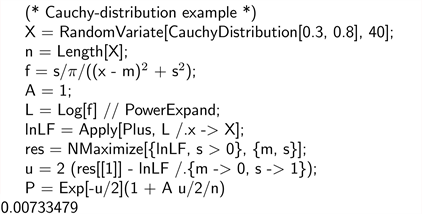
Based on the resulting P value, the null hypothesis would be rejected at 1% level of significance.

In our second example, we test whether parameters of a bivariate Normal distribution have the following values: ${\mu }_1={\mu }_2=0$ , ${\sigma }_1={\sigma }_2=1$ and $\rho =0.5$ (these are also the values we used to generate the sample of 100 bivariate observations).

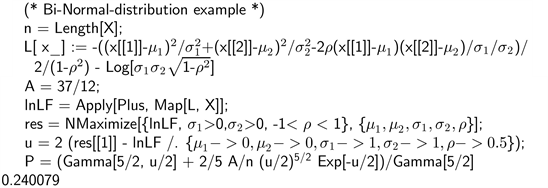
The resulting P value would lead to accepting the null hypothesis at any practical level of significance.

4. Accuracy Improvement

To investigate the accuracy of the new approximation, we need to be able to compute the level of confidence of the resulting region exactly. This can be done only in a few situations, such as the Exponential and Normal distributions. Exploring these two cases will give us a good indication of the improvement achieved by incorporating the A correction in general. The details of computing the exact confidence level may be of only passing interest to most readers; it is the resulting error tables which are important.

4.1. Exponential Case

We know that the ML estimator of the β parameter is given by the sample mean $\bar{X}$ whose exact distribution is Gamma(n, β/n). Since

$L\left(X\mathrm{<mo>\; ;\; </mo>}\beta \right)=-\frac{{\displaystyle {\sum }_{i=1}^n{X}_i}}{\beta }-n\ln \beta$ (34)

then

$2L\left(X\mathrm{<mo>\; ;\; </mo>}\bar{X}\right)-2L\left(X\mathrm{<mo>\; ;\; </mo>}\beta \right)=-2n\left(1+\ln \frac{\bar{X}}{\beta }-\frac{\bar{X}}{\beta }\right)$ (35)

(note that this expression is always non-negative, reaching a minimum value of zero when $\bar{X}=\beta$ ). The limits of the confidence interval of the basic technique are found by making (35) equal to a critical value of the ${\chi }_1^2$ distribution (let us call it $C_{\tau }$ , where $\tau$ is the corresponding level of confidence) and solving for $\bar{X}/\beta$ (and then, trivially, for $\beta$ ).

One can show that the two real solutions are given by

$-W_0\left(-\exp \left(-1-\frac{C_{\tau }}{2n}\right)\right)\text{and}-W_{-1}\left(-\exp \left(-1-\frac{C_{\tau }}{2n}\right)\right)$ (36)

where W is the Lambert (also called Omega, or “ProductLog” by Mathematica) function and the subscripts refer to its two real branches. To find the true confidence level, we need to integrate the PDF of $\bar{X}/\beta$ between these two limits (our code utilizes the corresponding CDF instead); subtracting the result from $\tau$ establishes the error of the basic algorithm. Further subtracting

$\frac{\sqrt{C_{\tau }}\exp \left(-\frac{C_{\tau }}{2}\right)}{6n\sqrt{\text{2}\pi }}$ (37)

then converts it into the error of our new formula (15). The following Mathematica program does that in four simple lines.

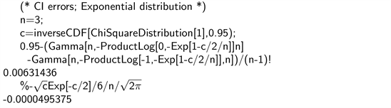
Both errors (using various sample sizes) are displayed in Table 2, using $\tau =95\%$ .

The table demonstrates that, as n increases, the error decreases with the first power of $\frac{1}{n}$ for the basic approximation, and with the second power of $\frac{1}{n}$ for our new algorithm.

4.2. Normal Case

Similarly, it is well known that the ML estimators of $\mu$ and ${\sigma }^2$ of the Normal distribution are $\bar{X}$ and $s^2:=\overline{X^2}-{\bar{X}}^2$ respectively, that they are independent of each other, and that their respective distributions are $N\left(\mu \mathrm{,}\frac{\sigma }{\sqrt{n}}\right)$ and Gamma( $\frac{n-1}{2},2{\sigma }^2$ ). Since

$L\left(X\mathrm{<mo>\; ;\; </mo>}\mu \mathrm{,}{\sigma }^2\right)=-\frac{{\displaystyle {\sum }_{i=1}^n{\left(X_i-\mu \right)}^2}}{2{\sigma }^2}-\frac{n}{2}\ln {\sigma }^2-n\ln \sqrt{2\pi }$ (38)

(1) then becomes

$2L\left(X\mathrm{<mo>\; ;\; </mo>}\bar{X}\mathrm{,}{s}^2\right)-2L\left(X\mathrm{<mo>\; ;\; </mo>}\mu \mathrm{,}{\sigma }^2\right)=-n\left(1+\ln \frac{s^2}{{\sigma }^2}-\frac{s^2}{{\sigma }^2}-\frac{{\left(\bar{X}-\mu \right)}^2}{{\sigma }^2}\right)$ (39)

To get the exact confidence level of the basic algorithm, we need to made this expression less than the critical value (denoted $C_{\tau }$ , as in the previous example) of the ${\chi }_2^2$ distribution, and integrate the joint PDF of $s^2/{\sigma }^2$ and $\sqrt{n}\left(\bar{X}-\mu \right)/\sigma$ over the resulting region. Solving the equation of its boundary for $s^2/{\sigma }^2$ in the manner of (35) now yields

$-W_0\left(-\exp \left(-1-\frac{C_{\tau }-Z^2}{n}\right)\right)\text{and}-W_{-1}\left(-\exp \left(-1-\frac{C_{\tau }-Z^2}{n}\right)\right)$ (40)

where Z stands for $\sqrt{n}\left(\bar{X}-\mu \right)/\sigma$ , having the standard Normal distribution.

Table 2. Aproximation errors (Exponential case).

We then integrate the PDF of $s^2/{\sigma }^2$ (having the ${\chi }_{n-1}^2$ distribution) using these two limits (again, the program utilizes the corresponding CDF instead); finally, we multiply the answer by the PDF of Z and integrate over all marginal values of Z (i.e. from 0 to $\sqrt{C_{\tau }}$ )—the last step is done numerically. This yields the true confidence level of the resulting confidence region; subtracting it from $\tau$ then provides the corresponding error of the basic algorithm; further subtracting

$\frac{C_{\tau }\exp \left(-\frac{C_{\tau }}{2}\right)}{24n}$ (41)

converts that into the error of the new algorithm. This is how it is done using Mathematica:

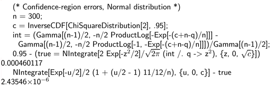
Table 3 summarizes the results.

Table 3. Approximation errors (Normal case).

Similarly to the previous example, one can clearly discern the $\frac{1}{n}$ -proportional decrease of the basic error, and the more rapid $\frac{1}{n^2}$ -proportional decrease achieved by our correction.

5. Conclusion

In this article, we have modified the traditional way (based on the corresponding likelihood function and a random independent sample of size n) of constructing a confidence region for distribution parameters, aiming to reduce its error. This has been achieved by adding, to the usual ${\chi }^2$ distribution of the original technique, a simple, $\frac{1}{n}$ -proportional correction whose coefficient is computed, for each specific distribution, using a rather complex formula; we have done the latter for many common distributions, summarizing the results in Table 1. We have also provided several examples of a Mathematica code, demonstrating the new algorithm and its simplicity (each computer program takes only a few lines); a practically identical approach can then be applied to the task of hypotheses testing. Finally, we have numerically investigated the improvement in accuracy thereby achieved, finding it rather substantial. It is worth emphasizing that, once the value of A has been established, incorporating the corresponding correction is extremely easy and done with a negligible computational cost.

Future research will hopefully explain why are the B and C coefficients of (29) both equal to zero; so far we have been able to prove that only by a brute-force computation, but we believe that there is some more fundamental reason behind this result, which we have not been able to uncover.

Conflicts of Interest

The author declares no conflicts of interest regarding the publication of this paper.

References

[1]	Kendall, M.G. and Stuart, A. (1969) The Advanced Theory of Statistics, Vol. 1, Chapter 3. Hafner Publishing Company, New York.
[2]	Bartlett, M.S. (1953) Approximate Confidence Intervals. Biometrica, 40, 12-19. https://doi.org/10.1093/biomet/40.1-2.12
[3]	Cysneiros, F.J.deA., dos Santos, S.J.P. and Cordeiro, G.M. (2001) Skewness and Kurtosis for Maximum Likelihood Estimator in One-Parameter Exponential Family Models. Brazilian Journal of Statistics and Probability, 15, 85-108.
[4]	Bowman, K.O. and Shenton, L.R. (1998) Aymptotic Skewness and the Distribution of Maximum Likelihood Estimators. Communications in Statistics—Theory and Methods, 27, 2743-2760. https://doi.org/10.1080/03610929808832252
[5]	Vrbik, J. (2013) Accurate Confidence Regions Based on MLEs. Advances and Applications in Statistics, 32, 33-56.
[6]	Vrbik, J. (2013) Addendum and Errata to “Accurate Confidence Regions Based on MLEs”. Advances and Applications in Statistics, 35, 161-163.