Hyperbolic Approximation on System of Elasticity in Lagrangian Coordinates ()
1. Introduction
Three most classical, hyperbolic systems of two equations in one-dimension are the system of isentropic gas dynamics in Eulerian coordinates
 (1)
(1)
where  is the density of gas,
  the velocity and
  the pressure; the nonlinear hyperbolic system of elasticity
 (2)
(2)
where  denotes the strain,
  is the stress and
  the velocity, which describes the balance of mass and linear momentum, and is equivalent to the nonlinear wave equation
 (3)
(3)
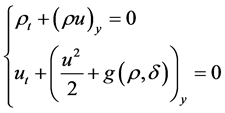
and the system of compressible fluid flow
 (4)
(4)
To obtain the global existence of weak solutions for nonstrictly hyperbolic systems (two eigenvalues are real, but coincide at some points or lines), the compensated compactness theory (cf. [1] [2] or the books [3] -[5] ) is still a powerful and unique method until now.
For the polytropic gas  where
where  and
and  is an arbitrary positive constant, the Cauchy problem (1) with bounded initial data was completely resolved by many authors (cf. [6] -[11] ). When
  has the same principal singularity as the
  -law in the neighborhood of vacuum
 , a compact framework was first provided in [12] [13] and later, the necessary
  compactness of weak entropy-entropy flux pairs for general pressure function was completed in [14] .
Under the strictly hyperbolic condition  and some linearly degenerate conditions
  or
or  as
as , the global existence of weak bounded solutions, or
  solutions,
  was obtained by Diperna [15] and Lin [16] , Shearer [17] respectively.
Without the strictly hyperbolic restriction, a preliminary existence result of the nonlinear wave Equation (3) was proved in [18] for the special case  under the assumption
  or
or .
.
Using the Glimm’s scheme method (cf. [19] ), Diperna [20] first studied the system (4) in a strictly hyperbolic region. Roughly speaking, for the polytropic case , Diperna’s results cover the case
 .
.
Since the solutions for the case of  always touch the vacuum, its existence was obtained in [21] by using the compensated compactness method coupled with some basic ideas of the kinetic formulations (cf. [10] [11] ). The existence of the Cauchy problem (7) for more general function
  was given in [22] under some conditions to ensure the
  compactness for all smooth entropy-entropy flux pairs.
If all smooth entropy-entropy flux pairs satisfy the  compactness, an ideal compactness framework to prove the global existence was provided by Diperna in [15] . For the above three systems (1)-(2) and (4), we can prove the
  compactness only for half of the entropies (weak or strong entropy).
2. Main New Ideas
In [14] (see also [23] for inhomogeneous system), the author constructed a sequence of regular hyperbolic systems
 (5)
(5)
to approximate system (1), where  in (5) denotes a regular perturbation constant and the perturbation pressure
 (6)
(6)
The most interesting point of this kind approximation is that both systems (5) and (1) have the same entropies (or the same entropy equation). In [14] , the  compactness of weak entropy-entropy flux pairs was also proved for general pressure function
 .
.
Let the entropy-entropy flux pairs of systems (1) and (5) be  and
and
 respectively. Then by using Murat-Tartar theorem, we have
 (7)
(7)
for any fixed , where the weak-star limit is denoted by
  as
as  goes to zero.
Paying attention to the approximation function (6), we know that
 (8)
(8)
are the entropy-entropy flux pairs of system
 (9)
(9)
or system
 (10)
(10)
respectively.
If we could prove from the arbitrary of  in (7) that
 (11)
(11)
and
 (12)
(12)
where  denotes the weak-star limit
  as
as  tend to zero, then we would have more function Equations (12) to reduce the strong convergence of
  as
as  tend to zero.
Between systems (2) and (4), we have the following approximation
 (13)
(13)
which has also the same entropy equation like system (2). If we could prove (11) and (12) from (7), then similarly we could prove the equivalence of systems (2) and (4). Moreover, we have much more information from system (13) to prove the existence of solutions for system (2) or (4).
Systems (13) and (2) have many common basic behaviors, such as the nonstrict hyperbolicity, the same entropy equation, same Riemann invariants and so on.
3. Main Results
By simple calculations, two eigenvalues of system (13) are
 (14)
(14)
with corresponding right eigenvectors
 (15)
(15)
and Riemann invariants
 (16)
(16)
Moreover
 (17)
(17)
and
 (18)
(18)
Any entropy-entropy flux pair  of system (13) satisfies the additional system
 (19)
(19)
Eliminating the  from (19), we have
 (20)
(20)
Therefore systems (13) and (2) have the same entropies. From these calculations, we know that system (13) is strictly hyperbolic in the domain  or
or , while it is nonstrictly hyperbolic on the domain
  since
since  when
when .
.
However, from (17) and (18), for each fixed , both characteristic fields of system (13) are genuinely nonlinear in the domain
  if
if  or in the domain
  if
if
 . In the first case
 , we have an a-priori
  estimate for the solutions of system (13)
 (21)
(21)
because the region

is an invariant region, where  (
( is given in Theorem 1),
  and
and  are positive constants depending on the initial date, but being independent of
 . In the second case
 , we have the
  estimate
 (22)
(22)
because the region

is an invariant region.
In this paper, for fixed , we first establish the existence of entropy solutions for the Cauchy problem (13) with bounded measurable initial data
 (23)
(23)
In a further coming paper, we will study the relation between the functions equations (11) and (12), and the convergence of approximated solutions of system (13) as  goes to zero.
Theorem 1 Suppose the initial data  be bounded measurable. Let (I):

where  is a positive constant, or (II):
 . Then the Cauchy problem (13)
with the bounded measurable initial data (23) has a global bounded entropy solution.
Note 1. The idea to use the flux perturbation coupled with the vanishing viscosity was well applied by the author in [24] to control the super-line, source terms and to obtain the  estimate for the nonhomogeneous system of isentropic gas dynamics.
Note 2. It is well known that system (2) is equivalent to system (1), but (1) is different from system (4) although the latter can be derived by substituting the first equation in (1) into the second. However, (4) can be considered as the approximation of (2). In fact, let  in (13). Then (13) is rewritten to the form
 (24)
(24)
for some nonlinear function .
.
Note 3. For any fixed , the invariant region
  above is bounded, so the vacuum is avoided. However, the limit of
 , as
, as  goes to zero, is the original invariant region of system (2) because
  could be infinity from the estimates in (21).
In the next section, we will use the compensated compactness method coupled with the construction of Lax entropies [25] to prove Theorem 1.
4. Proof of Theorem 1
In this section, we prove Theorem 1.
Consider the Cauchy problem for the related parabolic system
 (25)
(25)
with the initial data (23).
We multiply (25) by  and
and , respectively, to obtain
 (26)
(26)
and
 (27)
(27)
Then the assumptions on  yield
yield
 (28)
(28)
and
 (29)
(29)
if ; or
; or
 (30)
(30)
and
 (31)
(31)
if 
If we consider (28) and (29) (or (30) and (31)) as inequalities about the variables  and
and , then we can get the estimates
  by applying the maximum principle to (28) and (29) (or
 by applying the maximum principle to (30) and (31)). Then, using the first equation in (25), we get
  or
or  depending on the conditions on
 . Therefore, the region

or

is respectively an invariant region. Thus we obtain the estimates given in (21) or (22) respectively.
It is easy to check that system (13) has a strictly convex entropy when  or
or 
 (32)
(32)
We multiply (4.1) by  to obtain the boundedness of
 (33)
(33)
in . Then it follows that
 (34)
(34)
is bounded in . Since
  for some bounded constants
when  or
or , we get the boundedness of
 (35)
(35)
for any fixed .
.
Now we multiply (4.1) by , where
  is any smooth entropy of system (13), to obtain
 (36)
(36)
where  is the entropy-flux corresponding to
 . Then using the estimate given in (35), we know that the first term in the right-hand side of (36) is compact in
 , and the second is bounded in
 . Thus the term in the left-hand side of (36) is compact in
 .
.
Then for smooth entropy-entropy flux pairs  of system (13), the following measure equations or the communicate relations are satisfied
 (37)
(37)
where  is the family of positive probability measures with respect to the viscosity solutions
  of the Cauchy problem (25) and (23).
To finish the proof of Theorem 1, it is enough to prove that Young measures given in (37) are Dirac measures.
For applying for the framework given by DiPerna in [5] to prove that Young measures are Dirac ones, we construct four families of entropy-entropy flux pairs of Lax’s type in the following special form:
 (38)
(38)
 (39)
(39)
 (40)
(40)
 (41)
(41)
where  are the Riemann invariants of system (13) given by (16). Notice that all the unknown functions
  are only of a single variable
 . This special simple construction yields an ordinary differential equation of second order with a singular coefficient
  before the term of the second order derivative. Then the following necessary estimates for functions
  are obtained by the use of the singular perturbation theory of ordinary differential equations:
 (42)
(42)
 (43)
(43)
uniformly for  or
or , where
  and
and  is a positive constant independent of
 .
.
In fact, substituting entropies  into (20), we obtain that
 (44)
(44)
Let
 (45)
(45)
and
 (46)
(46)
Then
 (47)
(47)
The existence of  and its uniform bound
  on
on  or
or  with respect to
  can be obtained by the following lemma (cf. [26] ) (also see Lemma 10.2.1 in [15] ):
Lemma 2 Let  be the solution of the equation

and functions  be continuous on the regions

for some positive functions  and
and . In addition,


for some positive constants  and
and .
.
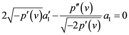
If  is a solution of the following ordinary differential equation of second order:

with  and
and  being arbitrary, then for sufficiently small
  and
and  ,
,  exists for all
  and satisfies

where 
Furthermore, we can use Lemma 2 again to obtain the bound of  with respect to
  if we differentiate Equation (46) with respect to
 .
.
By the second equation in (19), an entropy flux  corresponding to
  is provided by
 (48)
(48)
where
 (49)
(49)
if  or
or , and
, and  both are bounded uniformly on
  or
or .
.
In a similar way, we can obtain estimates on another three pairs of entropy-entropy flux of Lax type. Hence, Theorem 1 is proved when we use these entropy-entropy flux pairs in (38)-(41) together with the theory of compensated compactness coupled with DiPerna’s framework [15] .
5. Conclusions
In this paper we have looked at the general system of one-dimensional nonlinear elasticity in Lagrangian coordinates (2).
We construct a hyperbolic approximations to this which are parameterized by . They all have the same entropies as the original system. Under suitable assumptions we are able to establish uniform compactness estimates, and then obtain the existence of entropy solutions for the Cauchy problem.
Acknowledgements
This work was partially supported by the Natural Science Foundation of Zhejiang Province of China (Grant No. LY12A01030 and Grant No. LZ13A010002) and the National Natural Science Foundation of China (Grant No. 11271105).
NOTES
*Corresponding author.