A Direct Effective Viscosity Approach for Modeling and Simulating Bingham Fluids with the Cumulant Lattice Boltzmann Method

Martin Geier, Konstantin Kutscher, Manfred Krafczyk

Institute for Computational Modeling in Civil Engineering, TU Braunschweig, Braunschweig, Germany.

DOI: 10.4236/ojfd.2021.111003                

Abstract

Modeling of fluids with complex rheology in the lattice Boltzmann method (LBM) is typically realized through the introduction of an effective viscosity. For fluids with a yield stress behavior, such as so-called Bingham fluids, the effective viscosity has a singularity for low shear rates and may become negative. This is typically avoided by regularization such as Papanastasiou’s method. Here we argue that the effective viscosity model can be re-interpreted as a generalized equilibrium in which no violation of the stability constraint is observed. We implement a Bingham fluid model in a three-dimensional cumulant lattice Boltzmann framework and compare the direct analytic effective viscosity/generalized equilibrium method to the iterative approach first introduced by Vikhansky which avoids the singularity in viscosity that can arise in the analytic method. We find that both methods obtain similar results at coarse resolutions. However, at higher resolutions the accuracy of the regularized method levels off while the accuracy of the direct method continuously improves. We find that the accuracy of the proposed direct method is not limited by the singularity in viscosity indicating that a regularization is not strictly necessary.

Keywords

Lattice Boltzmann Method, Bingham Fluids, Generalized Equilibrium

1. Introduction

A popular way to model the stress of non-Newtonian fluids is by imposing an effective local viscosity. Unlike a Newtonian fluid with constant viscosity, this effective viscosity cannot be drawn in front of the gradient of the stress tensor of the Navier-Stokes equation. Implementing non-Newtonian fluids in Navier-Stokes solvers hence either requires storing the stress tensor explicitly or applying the chain rule to the effective viscosity field which can result in rather complicated differential operators. Being a method derived from kinetic theory, the cumulant LBM intrinsically stores the stress tensor separately from the primitive variables as second-order cumulants. Implementing non-Newtonian behavior through an effective viscosity thus comes naturally in the LBM with all differential operators applied in a consistent order.

Many substances of industrial interest are subject to non-Newtonian stress-strain relationships. One such example is fresh concrete [1]. The development of additive manufacturing techniques in civil engineering construction [2] depends critically on the availability of accurate and efficient numerical models for concrete. Among the many properties of freshly mixed concrete, the yield stress behavior is of particular importance in additive manufacturing processes which highly depends on a controlled transition from the fluid to the solid phase.

In this work we discuss the implementation of the Bingham fluid [3] in the context of the cumulant LBM [4]. The Bingham fluid model is a simple yield stress model with linear stress-strain relationship. Below the yield stress the Bingham fluid essentially behaves like a solid. In an effective viscosity approach this is modeled by assuming an essentially infinite viscosity. The transition between non-yielded and yielded behavior appears as a singularity in the effective viscosity model which apparently requires regularization. The most popular regularization is due to Papanastasiou [5] which relaxes the singularity by an exponential function. Ginzburg and Steiner [6] used Papanastasiou’s regularization to implement a Bingham fluid in the LBM. For computing the shear stress they used the non-equilibrium second-order moments which makes the method local and hence computationally efficient. However, for computing the shear stress locally in the LBM the viscosity has to be known. Ginzburg and Steiner used the local viscosity from the previous time step. Vikhansky [7] used an iterative method to recover the correct effective viscosity without further regularization. Tang et al. [8] introduced the He-Luo pressure based formulation [9] for a Bingham fluid in order to eliminate compressibility effects. For improved stability, Chen et al. implemented the Papanastasiou regularization in the multiple relaxation time (MRT) LBM framework. Further studies on Bingham fluids simulated with the LBM are described in [10] [11] [12]. Most of these works do not explicitly mention how the shear rate is numerically determined. However, the determination of the shear stress in the computation of the effective viscosity is an efficiency concern especially for large scale simulations. The local availability of the shear rate is one of the celebrated advantages of the LBM, but viscosity has to be known a priori to take advantage thereof. The two possibilities found in the above mentioned literature are either the one proposed by Ginzburg and Steiner using the viscosity of the previous time step or the one by Vikhansky solving an implicit relationship for each grid node at each time-step. From these two options the implicit one is more compelling as the use of a previous time step in an Eulerian setting can cause many problems. For example, if no advection equation for the viscosity is solved, the method cannot be Galilean invariant since the viscosity of a moving fluid is stored at a stationary grid. On the other hand, being fully explicit is often considered a computational advantage of the LBM. Being completely explicit implies (among other advantages) that the number of operations per time step is constant such that the wall clock time can be precisely predicted and, most importantly, maintained over the entire time simulated. This is by no means a minor concern, as the load balancing in high performance parallel computation relies heavily on the predictability of the run time of all subroutines. The works discussed above pay little to no attention to the parallel scalability of their approach. Most of them consider only two dimensional cases. In addition, none of these works use state of the art lattice Boltzmann kernels, but instead resort to simple single or multiple relaxation time variants.

In recent years, the LBM saw some significant evolution towards improved accuracy and stability. This improvement is due to the usage of tensor product lattices (i.e. using 27 discrete velocities in 3D), moment matching equilibria incorporating terms of higher than second-order in velocity, multiple relaxation times, Galilean invariant moment transformations (i.e. central moments or cumulants) and a better understanding of statistical independence of the different moments. These novel lattice Boltzmann methods include entropic schemes which typically implement tensor product lattices and tensor product equilibria and are primarily aimed at improving stability [13] [14] as well as central moment methods including so-called cascaded schemes [15] [16] [17] aiming particularly at improving Galilean invariance due to the observation that they are much more stable than moment methods in a static frame. Early multiple relaxation time methods [18] [19] did not pay proper attention to the correct segregation of moments and advocated the use of orthogonal transformation matrices. Even though, some early method used a more appropriate weighted orthogonality condition [20], it is comparatively recent that the requirement of statistical independence between observable quantities relaxing with different relaxation times has been appreciated. The cumulant model is based on the statistical independence concept [4] [21] [22] [23]. It incorporates all of the above mentioned recent developments improving both stability and accuracy of the LBM.

In this paper we present an implementation of the Bingham fluid in the context of the cumulant LBM. Our approach starts similar to the one of Vikhansky [7]. We observe that the implicit problem solved iteratively by Vikhansky actually has an analytic solution. However, this analytic solution has a singularity in viscosity which manifests in a violation of the linear stability constraint of the LBM. Surprisingly, this violation is avoided by the approximate solution of Vikhanski even at arbitrary iteration depth. That is to say, the approximate solution does not converge to the analytic solution at positions where the analytic solution is not physically meaningful. Using the approximate solution can hence be regarded as a special form of regularization. However, to the best of our knowledge the unregularized analytic solution of the implicit problem has never been systematically compared to the approximate solution. With its violation of the linear stability constraint, the analytic solution could be expected to yield unstable results. This, however, is not observed to be the case. In this paper we show that the effective viscosity ansatz can be reinterpreted as a generalized equilibrium approach for which no violation of stability is indicated.

We test our model with two simple planar flows: the flow between two infinite plates and the flow between a rotating and a stationary cylinder. Even though these cases are relatively simple, they both cover the singularity problem of the effective viscosity and include extended areas in which the fluid is expected to behave as a solid.

In the following, we will briefly introduce the cumulant LBM, discuss the implementation of the Bingham fluid and the regularization including a fixed-point iteration scheme which removes the singularity. Next we will discuss an alternative interpretation of the effective viscosity model as a generalized equilibrium model in which the singularity disappears. This is followed by a numerical comparison between the two possibilities and conclusions.

2. Cumulant Lattice Boltzmann Model

The effective viscosity of non-Newtonian fluids can vary substantially such that it is imperative to use a model base with a large range of attainable viscosities. Early lattice Boltzmann models based on single relaxation time collision operators [24] had a rather limited range of viscosity due to stability issues. In the last two decades substantial progress has been made, in particular regarding the extension of LBM to lower viscosity limits. It is of note that by proper scaling of the grid spacing and the time step any consistent numerical method with limited stability can, in principle, model any viscosity. However, if viscosity is not constant throughout the domain, the ratio between the smallest and the largest attainable viscosity determines which viscosity range can effectively be simulated. Therefore, it is important for the underlying fluid solver for non-Newtonian fluids to have good accuracy and stability properties over a large range of viscosities. In this paper we use the cumulant LBM [4] which is among the LBM with the largest stability range as well as with the highest accuracy for the given D3Q27 stencil used. The cumulant LBM discretizes the Boltzmann equation in the hydrodynamic limit. It is a discrete velocity model using 27 discrete speeds on a tensor product lattice. The discrete velocity distribution function $f_{ijk}$ streams along the discrete velocity directions $i{\stackrel{\to }{e}}_x+j{\stackrel{\to }{e}}_y+k{\stackrel{\to }{e}}_z$ in discrete time steps $\Delta t$ from lattice node to lattice node. At lattice nodes the distribution undergoes a local collision which is performed in cumulant space. Cumulants are the statistically independent observable quantities of a statistical distribution. Previous lattice Boltzmann models either applied the collision operator directly in distribution space [24] or in moment space [18]. Moments can be defined in a large variety of ways [25]. Important properties of a moment base are the chosen frame of reference (e.g. Eulerian leading to raw moments or Lagrangian implying central moments), their orthogonality properties ((non-)orthogonal, weighted orthogonal (i.e. Hermite moments)), and their grouping according to symmetry properties (rotational invariance). Performing collisions in moment or cumulant space allows for a substantially improved control of the properties of the method as different quantities can evolve on different time scales when using different relaxation times. However, for this to be consistent, the different moments have to be statistically independent. Traditionally this is attempted to be enforced by orthogonalization. However, orthogonalization has no unique definition for moments. Moments orthogonal in one frame of reference are not orthogonal in another frame of reference. Even in a Lagrangian frame of reference, moments which are orthogonal in equilibrium are not orthogonal when out of equilibrium. Cumulants overcome this inconsistency as they are derived from the definition of statistical independence.

The cumulant collision operator assigns an individual relaxation rate ${\omega }_{abc}$ to each cumulant $C_{abc}$ such that the post collision cumulants $C_{abc}^{\ast }$ can be computed as:

$C_{abc}^{\ast }=C_{abc}+{\omega }_{abs}\left(C_{abc}^{eq}-C_{abc}\right)$ (1)

where the equilibrium cumulant $C_{abc}^{eq}$ is typically zero for non-conserved cumulants but can also be chosen otherwise in certain circumstances, for example if energy conservation is not considered as is usually the case for the incompressible Navier-Stokes equation. Asymptotic analysis [26] of the lattice Boltzmann equation reveals two relationships of interest for the modeling of non-Newtonian fluids.

The viscosity is related to the relaxation rate of second-order cumulants (i.e. $\omega ={\omega }_{110}={\omega }_{101}={\omega }_{011}$ and the corresponding diagonal terms of second-order of the tensor ${\omega }_{abc}$ with the exception of the trace):

$\nu =\frac{1}{3}\left(\frac{1}{\omega }-\frac{1}{2}\right)\frac{\Delta x^2}{\Delta t}$ (2)

The shear stress in the LBM can be written as:

$\tau =\nu \rho \stackrel{\dot{}}{\gamma }$ (3)

For a known viscosity the shear rate can be locally computed from the second-order cumulants:

$\stackrel{\dot{}}{\gamma }=\frac{\partial u_i}{\partial x_j}+\frac{\partial u_j}{\partial x_i}$ (4)

$\frac{\partial u_1}{\partial x_2}+\frac{\partial u_2}{\partial x_1}=\frac{\omega }{3\rho }{C}_{110}$ (5)

$\frac{\partial u_1}{\partial x_1}-\frac{\partial u_2}{\partial x_2}=\frac{2\omega }{3\rho }\left(C_{200}-C_{020}\right)$ (6)

Here we omitted the other permutations of Equations (5) and (6).

The LBM does not require any additional finite differencing for the calculation of the shear rate. However, it is of note that the relaxation time, which is a function of viscosity, appears in the equations for the shear rate such that an implicit problem arises if the viscosity depends on the shear rate.

3. Bingham Fluid

The Bingham fluid [3] extends a Newtonian fluid by a constant yield stress ${\tau }_0$ :

${\tau }_{Bing}={\tau }_0+{\nu }_{\infty }\rho \stackrel{\dot{}}{\gamma }$ (7)

Our aim is to impose Equation (7) onto the LBM. This is done through equating Equations (3) and (7):

${\tau }_0+{\nu }_{\infty }\rho \stackrel{\dot{}}{\gamma }=\nu \rho \stackrel{\dot{}}{\gamma }$ (8)

$\frac{{\tau }_0}{\rho }+\frac{\stackrel{\dot{}}{\gamma }}{3}\left(\frac{1}{{\omega }_{\infty }}-\frac{1}{2}\right)\frac{\Delta x^2}{\Delta t}=\frac{\stackrel{\dot{}}{\gamma }}{3}\left(\frac{1}{\omega }-\frac{1}{2}\right)\frac{\Delta x^2}{\Delta t}$ (9)

According to Equation (5) $\stackrel{\dot{}}{\gamma }$ is a function of $\omega$. To make this relationship explicit, we define:

${\stackrel{\dot{}}{\gamma }}_{\infty }=\stackrel{\dot{}}{\gamma }\left({\omega }_{\infty }\right)$ (10)

$\stackrel{\dot{}}{\gamma }\left(\omega \right)={\stackrel{\dot{}}{\gamma }}_{\infty }\frac{\omega }{{\omega }_{\infty }}$ (11)

With this Equation (9) can be stated as:

$\frac{{\tau }_0}{\rho }+\frac{{\stackrel{\dot{}}{\gamma }}_{\infty }}{3}\left(\frac{1}{{\omega }_{\infty }}-\frac{1}{2}\right)\frac{\Delta x^2}{\Delta t}\frac{\omega }{{\omega }_{\infty }}=\frac{{\stackrel{\dot{}}{\gamma }}_{\infty }}{3}\left(\frac{1}{\omega }-\frac{1}{2}\right)\frac{\Delta x^2}{\Delta t}\frac{\omega }{{\omega }_{\infty }}$ (12)

This can be solved for the relaxation rate to give explicitly:

${\omega }_a={\omega }_{\infty }\left(1-\frac{3{\omega }_{\infty }{\tau }_0\Delta t}{{\stackrel{\dot{}}{\gamma }}_{\infty }\rho \Delta x^2}\right)$ (13)

We will call the relaxation rate in Equation (13) the analytic relaxation rate ${\omega }_a$. Apparently Equation (13) allows us to simulate a Bingham fluid using only local operations as in a standard Newtonian LBM solver. However, we observe that ${\omega }_a$ remains in the range for linear stability ${\omega }_a\in \left\{0\cdots 2\right\}$ only for ${\stackrel{\dot{}}{\gamma }}_{\infty }\rho <3{\omega }_{\infty }{\tau }_0$. According to Equation (2) viscosity goes to infinity when $\omega =0$ and viscosity will be negative for $\omega <0$. Regularization procedures like the one by Vikhansky [7] are imposed to avoid the singularity in viscosity.

3.1. Regularization

From Equation (8) it is not obvious why the effective viscosity $\nu$ should become negative before the shear rate $\stackrel{\dot{}}{\gamma }$ reaches zero. The reason for the problem encountered in the last subsection is in the implicit dependence of $\stackrel{\dot{}}{\gamma }$ on the relaxation rate when computed from the second-order cumulants. If we ignore this implicit dependence and solve Equation (9) for $\omega$ we obtain:

$\omega =\frac{{\omega }_{\infty }\stackrel{\dot{}}{\gamma }\rho \Delta x^2}{\Delta x^2\stackrel{\dot{}}{\gamma }\rho +3{\omega }_{\infty }{\tau }_0\Delta t}$ (14)

This solution is always positive, but it requires $\stackrel{\dot{}}{\gamma }$ which in lattice Boltzmann is only known through $\stackrel{\dot{}}{\gamma }={\stackrel{\dot{}}{\gamma }}_{\infty }\omega {\omega }_{\infty }^{-1}$. Instead of using the apparently unfeasible analytic solution, we can solve Equation (14) through a fixed-point iteration as follows [7]:

${\omega }_0={\omega }_{\infty }$ (15)

${\omega }_{n+1}=\frac{{\omega }_{\infty }{\stackrel{\dot{}}{\gamma }}_{\infty }{\omega }_n\rho \Delta x^2}{\Delta x^2{\stackrel{\dot{}}{\gamma }}_{\infty }{\omega }_n\rho +3{\omega }_{\infty }^2{\tau }_0\Delta t}$ (16)

Since all terms on the right hand side of Equation (16) are positive and since we start the iteration from a positive value ${\omega }_{n+1}$ is always guaranteed to be positive.

In order to accelerate the execution of the fixed-point iteration we rewrite Equation (16):

$\frac{{\omega }_{\infty }}{{\omega }_{n+1}}=1+\frac{3{\omega }_{\infty }{\tau }_0\Delta t}{{\stackrel{\dot{}}{\gamma }}_{\infty }\rho \Delta x^2}\frac{{\omega }_{\infty }}{{\omega }_n}=1+A\frac{{\omega }_{\infty }}{{\omega }_n}$ (17)

We note that Equation (17) has a simple analytic solution for ${\omega }_{n+1}={\omega }_n$ which can easily be verified to be identical with Equation (13) which we are trying to avoid. In fact a solution of Equation (17) exists only for ${\omega }_n\ne 0$ which is the mathematical reason for the analytic solution appearing to be unfeasible.

The obtained iteration can be easily unrolled for a fixed iteration depth. For example, the iteration of depth five reads:

${\omega }_5=\frac{{\omega }_{\infty }}{1+A\left(1+A\left(1+A\left(1+A\left(1+A\right)\right)\right)\right)}$ (18)

In his original paper [7] Vikhansky claims that two to three iterations are sufficient to reach convergence. However, it is unclear to us whether he started from the relaxation rate of the previous time step which would certainly reduce the number of iterations but would come at additional cost in memory consumption and data transfer and would not be Galilean invariant. It is of note that the fixed-point iteration is not expected to converge quickly. The convergence order can be computed directly by comparing two subsequent iterations:

$\frac{{\omega }_{n+1}}{{\omega }_n}=\frac{1}{1+A}$ (19)

The rate of change is constant implying linear convergence. However, we should remind ourselves that we deliberately replaced the exact solution by this approximation for the purpose of regularization and avoiding the singularity of the exact solution. The use of faster converging methods like Aitken extrapolation or Newton iteration would reintroduce the possibility for the relaxation rate to become negative and could hence eliminate the advantage of regularization. That is, of course, if regularization is really as advantageous as implied through the avoidance of the singularity in viscosity.

Naively, one could assume that a singularity in viscosity and the violation of the linear stability regime should result in unstable simulations. However, in the current case, as demonstrated below, this problem did not manifest in our simulations. A simple reason why the violation of the linear stability constraint might not be relevant in the current case is seen from the fact that according to Equation (13) a problem occurs only if the shear rate is small enough. Instability would necessarily manifest itself in a locally increased shear rate which would force the relaxation rate back into its stable range. Thus, even though the linear stability constrained is violated, this violation is self-limiting and consequently non-linearly stable.

We also have to take the nature of the LBM into consideration and how it compares to a classical Navier-Stokes solver. In a classical Navier-Stokes solver the stress tensor is constructed by computing the shear rate and multiplying it with the viscosity. A singularity in viscosity is numerically unmanageable in this context and obviously has to be avoided. However, in the LBM, viscosity is an emergent property of the relaxation rate. The singularity occurs when $\omega =0$ which is not necessarily a problem for the lattice Boltzmann algorithm itself as it does not divide by $\omega$. The problem of a singular viscosity is hence a very serious numerical difficulty for the Navier-Stokes equation, but it is not necessarily relevant for the LBM.

It is instructive to recall that the effective viscosity ansatz is only an algebraic trick to express the yield stress through the relaxation rate. Alternatively we could specify the yield stress in the equilibrium second-order cumulants and leave the relaxation rates untouched. A similar dual approach exists in the correction for cubic error terms in viscosity of the LBM. Dellar [27] decided to incorporate this correction into a modified relaxation rate while we implemented it by a modified equilibrium function of second-order cumulants [4]. Even though these approaches appear to be rather different in concept, a detailed investigation shows that both methods are algebraic transformations of each other and should hence yield identical results up to round-off errors. In the following we demonstrate the equivalence of the modified relaxation rate to a generalized equilibrium.

3.2. Equivalence of Effective Relaxation Rate and Generalized Equilibrium Approaches

Asymptotic analysis as, for example, demonstrated in appendix G of [4] can be used to calculate the relationship between second-order cumulants and the velocity derivatives:

$\frac{\partial u_1}{\partial x_2}+\frac{\partial u_2}{\partial x_1}=\frac{\omega }{3\rho }\left(C_{110}-C_{110}^{eq}\right)$ (20)

$\frac{\partial u_1}{\partial x_1}-\frac{\partial u_2}{\partial x_2}=\frac{2\omega }{3\rho }\left(C_{200}-C_{020}-C_{200}^{eq}+C_{020}^{eq}\right)$ (21)

Note that Equation (20) and (21) are identical to Equation (5) and (6), respectively (up to an unspecified equilibrium cumulant each). The equilibrium here is understood as a generalized equilibrium as introduced by Asinari [28] for analyzing the cascaded LBM. The generalized equilibrium is an attractor for the collision operator and does not necessarily have a direct thermodynamic interpretation. For the respective second-order cumulants the thermodynamic equilibria would be zero which is why they are omitted from Equations (5) and (6). Here we include them for the purpose of showing that an effective relaxation rate can be equivalently understood as a generalized equilibrium. For this purpose we consider Equation (5) with the equivalent relaxation rate ${\omega }_a$ resulting from the rheology model and the fixed Newtonian relaxation rate ${\omega }_{\infty }$ :

$\frac{\partial u_1}{\partial x_2}+\frac{\partial u_2}{\partial x_1}=\frac{{\omega }_a}{3\rho }{C}_{110}$ (22)

$=\frac{{\omega }_{\infty }}{3\rho }\left(C_{110}-\frac{{\omega }_{\infty }-{\omega }_a}{{\omega }_{\infty }}{C}_{110}\right)$ (23)

$C_{110}^{eq}=\frac{{\omega }_{\infty }-{\omega }_a}{{\omega }_{\infty }}{C}_{110}$ (24)

It is hence seen that the equivalence between the modified relaxation rate in Equation (22) and the generalized equilibrium at fixed relaxation rate in Equation (22) is established by choosing the specific equilibrium Equation (24). It is of particular note here that this relationship is independent of how ${\omega }_a$ was obtained in the first place, implying that any method using an effective relaxation rate can be rewritten as a method with fixed relaxation rate and generalized equilibrium. This hence applies to Vikhansky’s model for Bingham fluids [7] in the same way as for Dellar’s Galilean correction to the viscosity [27]. The inverse, however, is not true as we see that the generalized equilibrium depends on the cumulant itself implying that only generalized equilibria of a very specific form can be turned into an effective relaxation rate.

In the generalized equilibrium form, the linear stability constraint is not necessarily violated if ${\omega }_a<0$. It hence seems to be admissible to use the analytic solution of the effective relaxation rate even if it might become negative.

4. Curved Boundary Conditions

Being a Cartesian grid based method, the LBM is applicable to real world industrial problems only because effective methods to incorporate grid refinement and curved boundary conditions have been incorporated. Most of these methods are dependent on the local viscosity and their application to non-Newtonian fluids requires some adjustment. We leave the important topic of grid refinement to future work and discuss the implementation of an off-grid velocity boundary conditions applicable to moving curved walls.

In lattice Boltzmann, velocity boundary conditions are conveniently implemented via a bounce back scheme with modified velocity. Bounce back is applied on links entering the fluid domain during the streaming step. In its simplest implementation, bounce back returns the population leaving the domain as the population entering the domain in opposite direction. This results in a zero velocity boundary condition approximately halfway between grid nodes. The no-slip (i.e. bounce back) boundary is turned into a velocity boundary condition by adding twice the momentum of the moving wall [29]:

$f_{\bar{i}\bar{j}\bar{k}}^{BB}\left(\stackrel{\to }{x},t+\Delta t\right)=f_{ijk}^{\ast }\left(\stackrel{\to }{x},t\right)+\frac{2w_{ijk}\rho {\stackrel{\to }{e}}_{ijk}\cdot {\stackrel{\to }{u}}^{BC}}{c_s^2}$ (25)

Here $f^{\ast }\left(\stackrel{\to }{x}\mathrm{,}t\right)$ is the post-collision state of the boundary node at the previous time step. The over bar denotes the direction opposite to the boundary. Further we used the lattice weights $w_{ijk}$ ( $w_{100}=2/27$, $w_{110}=1/54$, $w_{111}=1/216$ ) and so on by permuting indices) and the link direction ${\stackrel{\to }{e}}_{ijk}$.

For industrial applications it would be unacceptable that boundaries had to be set halfway between grid nodes. For this reason, interpolation bounce back schemes have been popular for quite some time [30] [31] [32]. For the implementation of an interpolation boundary condition, a sub-grid distance $q\Delta x$, $q\in \left\{0\cdots 1\right\}$ has to be specified for each link cutting into the boundary. For $q=0$ the boundary coincides with the grid node at which the boundary is applied. If $q=1$ the boundary is at the neighboring node and for other values the boundary is located in between. Interpolation boundary conditions usually require several grid nodes for the interpolation stencil. In lattice Boltzmann, everything which is not local in space is considered to be inefficient as it complicates data structures and domain decomposition for parallel computing. It is hence desirable to implement boundary conditions of similar accuracy using only locally available data. Fortunately, this is possible in LBM by interpolating between pre- and post-collision distributions (see appendix E in [4] ). To see this we consider the relationship between the post-collision state of the distribution leaving the domain and the pre-collision state at the node beyond the boundary:

$f_{ijk}\left(\stackrel{\to }{x}+{\stackrel{\to }{e}}_{ijk}\Delta x\mathrm{,}t+\Delta t\right)=f_{ijk}^{\ast }\left(\stackrel{\to }{x}\mathrm{,}t\right)$ (26)

Instead of interpolating in space only, as done by the classical interpolated bounce back scheme, it is possible to interpolate in space and time towards the boundary:

$f^{BC}\left(\stackrel{\to }{x}+q{\stackrel{\to }{e}}_{ijk}\Delta x\mathrm{,}t+q\Delta t\right)=q{f}_{ijk}\left(\stackrel{\to }{x}\mathrm{,}t\right)+\left(1-q\right)f_{ijk}^{\ast }\left(\stackrel{\to }{x}\mathrm{,}t\right)$ (27)

At the boundary the bounce back or velocity bounce back method according to Equation (25) can be applied to recover $f_{\bar{i}\bar{j}\bar{k}}^{BB}$. Next to the boundary the incoming distributions are recovered by interpolation from the distributions leaving the boundary node in the direction opposite to the boundary:

$f_{\bar{i}\bar{j}\bar{k}}\left(\stackrel{\to }{x}\mathrm{,}t+2q\Delta t/\left(q+1\right)\right)=\frac{f_{\bar{i}\bar{j}\bar{k}}^{BB}\left(\stackrel{\to }{x}+q{\stackrel{\to }{e}}_{ijk}\Delta x\mathrm{,}t+q\Delta t\right)}{q+1}+\frac{q{f}_{\bar{i}\bar{j}\bar{k}}^{\ast }\left(\stackrel{\to }{x}\mathrm{,}t\right)}{q+1}$ (28)

It is observed that the population arrives at the correct location. However it appears to arrive at the wrong time instance $t+2q\Delta t/\left(q+1\right)$ instead of at $t+\Delta t$. This is of minor concern as the LBM recovers the Navier-Stokes equation only in diffusive scaling $\Delta t\propto \Delta x^2$. A first-order scheme in time is as accurate as a second-order scheme in space. Since the linear interpolation is already second-order in space, the first-order interpolation in time does not increase the error asymptotically compared to the classical interpolation method using several nodes. By using pre- and post-collision states, the boundary condition either requires the presence of both states or it has to compute and apply the collision operator in the boundary. Modern implementations of the LBM using in-place streaming methods like EsoTwist [33] keep only a single representation of the distribution function values in memory at any time which saves essentially 50% of the memory required for standard implementations. Considering computational efficiency, it is usually preferable to repeat the collision step at a limited number of boundary nodes rather than to double the memory requirements in the entire domain. A considerable simplification is obtained by replacing the cumulant collision operator by the single relaxation time collision operator at the boundary. The latter requires only the local equilibrium function $f_{ijk}^{eq}$ and can be computed as:

$f_{ijk}^{\ast }=f_{ijk}+\left(1-\omega \right)\left(f_{ijk}-f_{ijk}^{eq}\right)$ (29)

The non-Newtonian fluid model enters the boundary condition only in the determination of $\omega$. This can be implemented for the iterative as well as for the analytic model of the Bingham fluid’s viscosity.

5. Implementation Details

The Bingham fluid model with unrolled iterative regularization according to Equation (18) and the method based on the analytic solution are implemented in the massively parallel lattice Boltzmann solver Virtual Fluids [34]. The base model is the cumulant lattice Boltzmann solver with 27 velocities and optimized relaxation rates as introduced in [35] and analyzed in [36] [37]. In this method, the relaxation rates of cumulants of order three and higher are selected depending on the relaxation rates of second-order cumulants and this optimization is only valid in a specific range of relaxation rates associated with low viscosity. For the high viscosity encountered below the yield threshold the optimization would introduce additional singularities in the higher cumulants. This is avoided here by selecting the relaxation rates of the higher-order cumulants according to the fixed asymptotic relaxation rate ${\omega }_{\infty }$ which means that we are applying the generalized equilibrium instead of the effective viscosity ansatz. A caveat to this choice is that ${\omega }_{\infty }$ is somewhat arbitrary such that the optimization obtained in [35] for Newtonian fluids might not be optimal for non-Newtonian fluids. However, the complex optimization procedure in [35] heavily relies on the linearization of the LBM and requires substantial further research to be fully applied to the non-linearity of the Bingham fluid. We will hence leave a Bingham specific optimization of the relaxation rates to future research.

The lattice Boltzmann algorithm including the computation of the effective relaxation rate for boundary conditions and the collision operator is given in Algorithm 1.

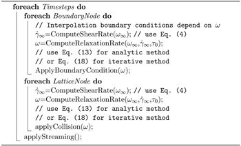
Algorithm 1. Lattice Boltzmann algorithm for Bingham uids.

6. Numerical Validation

The main purpose of the current paper is to demonstrate that the viscosity singularity which has to be avoided in Navier-Stokes implementations of the effective viscosity model does not arise in the LBM. For demonstration purpose we chose two canonical test cases which are both popular and relevant for Bingham fluids: Poiseuille flow and Taylor-Couette flow. Yet, even for these comparatively simple setups proper convergence studies for yield stress fluids are rarely found in literature.

6.1. Poiseuille Flow

A classical and simple test for the implementation of a Bingham fluid is flow between two infinite plates driven by a constant force. This Poiseuille type flow results in a parabolic flow near the boundaries and a plug flow in the center of the channel for a Bingham fluid as described in [38]:

$u_x=\{\begin{array}{l}\frac{1}{2}{\left(\frac{F_x}{\mu }\right)}^{\frac{1}{2}}{\left(H-z_0\right)}^2\mathrm{,}0\le z\le z_0\\ \frac{1}{2}{\left(\frac{F_x}{\mu }\right)}^{\frac{1}{2}}\left({\left(H-z_0\right)}^2-{\left(z-z_0\right)}^2\right)\mathrm{,}{z}_0\le z\le H\end{array}$ (30)

where $F_x$ is the force amplitude driving the flow, $z_0$ is the yield point given by $z_0=\frac{{\tau }_0}{F_x}$, H is the half height of the channel and $\mu =\rho \nu$ is the dynamic

viscosity. Driving the flow by a force $F_x$ is typically preferred in benchmark simulations over the more physically correct pressure gradient as the latter cannot be implemented with periodic boundaries and would hence introduce boundary effects from the pressure boundary conditions.

We used a simulation domain of size $2\times 2H\times 2$. The viscosity at the lowest resolution $\mu$ was set to 0.005, the yield stress ${\tau }_0=3\times {10}^{-8}$ and the force was $F_x=6\times {10}^{-9}$. As usual in LBM literature, all quantities here are given in normalized lattice units where we assume that grid spacing, time step and mass element are all unity, i.e. $\Delta x=1$, $\Delta t=1$ and $\Delta m=1$. For studying the convergence we varied the resolution of the problem for fixed Mach, Reynolds and Bingham numbers defined respectively as:

$Ma=\frac{U}{c_s}$ (31)

$Re=\frac{\rho UH}{\mu }$ (32)

$Bm=\frac{{\tau }_{0}H}{\mu U}$ (33)

The speed of sound $c_s\mathrm{<mo>\; =\; </mo>}\sqrt{1/3}\Delta x\Delta t^{-1}$ is a constant in the LBM such that consistency between the dimensionless numbers is established by scaling ${\mu }_{\star }=\mu \Delta x/\Delta x_{\star }$ and $F_{x\star }=F_x\Delta x_{\star }/\Delta x$. This scaling implies that the time step $\Delta t$ is scaled proportionally to the grid spacing $\Delta x$ which also keeps the velocity scale U constant. The disadvantage of this so-called acoustic scaling is that a finite error in Mach number persists such that absolute convergence is not expected. In order for this to be small we chose rather small values for the force and the yield stress.

To quantify the error we compute the following L2 norm

${\Vert u_x-u_x^a\Vert }_{L2}=\sqrt{\frac{{\displaystyle \sum }{\left(u_x-u_x^a\right)}^2}{{\displaystyle \sum }{\left(u_x^a\right)}^2}}$ (34)

Figure 1 shows the velocity profile of the channel flow for the Bingham fluid simulated with the analytic function for the relaxation rate ( ${\omega }_a$ ) and the approximated solution using 20 iterations ( ${\omega }_{20}$ ). The figure implies satisfactory correspondence of both solutions with the analytic solution. Differences between both methods become visible in the L2 norm seen in Figure 2. It is observed that neither methods convincingly displays second-order convergence down to a resolution of 256 lattice nodes in the span. While both methods give nearly identical results for the lowest resolution, the approximate method levels off at higher resolutions.

(a) (b)

Figure 1. Velocity profile of the Bingham fluid using four different resolutions. The left plot (a) shows results obtained using the analytic relaxation rate while the right plot (b) shows result for the iterative method using 20 iterations. The value of H given in lattice units indicates the resolution. Between 32 and 256 nodes across the span of the channel were used in this convergence study. (a) Analytic relaxation; (b) Iterative relaxation.

Figure 2. Convergence of the L2 norm for the flow shown in Figure 1. The dashed line indicates second-order convergence.

6.2. Taylor-Couette Flow

Our next test is a planar Taylor-Couette flow depicted in Figure 3. We investigate the flow between a rotating outer and a resting inner cylinder. Perpendicular to the plane periodic boundary conditions are used such that the setup is quasi two dimensional. Interpolated bounce back with and without velocity is used for the outer and the inner cylinder, respectively. In this test case, flow attached to the outer cylinder will be below the yield threshold and hence move as a solid with the same angular velocity as the outer cylinder. This plug flow domain attached to the outer cylinder is reduced in size with higher angular momentum.

6.2.1. Semi-Analytic Solution

A semi-analytic solution for the laminar Taylor-Couette flow of a Bingham fluid is usually derived in dimensionless form scaled with the Reynolds number of the inner cylinder [39] [40]. This unfortunately precludes the case where the inner cylinder is at rest. We hence present here a semi-analytic solution for this particular case. Following Landry et al. [40] we start from the condition for stationary momentum in cylindrical coordinates:

$0=\frac{1}{r^2}\frac{\partial }{\partial r}\left(r^2{\tau }_{r\theta }\right)$ (35)

The stress in the Bingham fluid is given in cylindrical coordinates as:

${\tau }_{r\theta }=\left(\mu +\frac{{\tau }_0}{\left|{\stackrel{\dot{}}{\gamma }}_{r\theta }\right|}\right){\stackrel{\dot{}}{\gamma }}_{r\theta }$ (36)

${\stackrel{\dot{}}{\gamma }}_{r\theta }=\{\begin{array}{l}0,\left|{\tau }_{r\theta }\right|\le {\tau }_0\\ \frac{\text{d}V\left(r\right)}{\text{d}r}-\frac{V\left(r\right)}{r},\left|{\tau }_{r\theta }\right|>{\tau }_0\end{array}$ (37)

where $V\left(r\right)$ is the tangential velocity at radius r. For the purpose of this derivation we assume $\left|{\tau }_{r\theta }\right|>{\tau }_0$ and plug Equation (36) into Equation (35). This gives rise to a 2nd order ordinary differential equation which we supplement

Figure 3. Concept of Taylor-Couette flow with Bingham fluid. An outer ring with finite thickness where the stress is below the yield threshold rotates like a solid body with the outer wall.

with two boundary conditions. Unlike Bird et al. [39] and Landry et al. [40] we consider the case of a resting inner cylinder, i.e. $V\left(R_i\right)=0$ and a moving outer cylinder. For the boundary condition imposed by the outer cylinder we have to take our assumption of $\left|{\tau }_{r\theta }\right|>{\tau }_0$ into consideration, meaning that the differential equation is not valid beyond the yield radius $R_y$. At the yield radius and beyond the fluid moves as a solid with the angular velocity of the outer cylinder such that we can specify the boundary condition $V\left(R_y\right)=\Omega R_y$. This gives rise to the analytic solution

$V\left(r\right)=\{\begin{array}{l}\frac{\mu \Omega {\mathcal{R}}_{\alpha }^2+{\tau }_0{\mathcal{R}}_{\beta }^2\ln \left(\frac{r}{R_y}\right)-{\tau }_0{\mathcal{R}}_{\gamma }^2\ln \left(\frac{R_i}{R_y}\right)}{\mu r\left(R_i^2-R_y^2\right)},R_i<r\le R_y\\ r\Omega ,r>R_y\end{array}$ (38)

With

${\mathcal{R}}_{\alpha }^2=\left(R_i^2-r^2\right)R_y^2$ (39)

${\mathcal{R}}_{\beta }^2=\left(R_y^2-R_i^2\right)r^2$ (40)

${\mathcal{R}}_{\gamma }^2=\left(R_y^2-r^2\right)R_i^2$ (41)

The yield radius $R_y$ is unknown and it is recovered from the condition of continuity for Equation (37). Basically we need to solve

$0=\frac{\text{d}V\left(R_y\right)}{\text{d}{R}_y}-\frac{V\left(R_y\right)}{R_y}$ (42)

for $R_y$. This is done here numerically such that the final solution is only semi-analytic. As there are multiple solutions we have to pick the one for which $R_y>R_i$.

6.2.2. Results

Figure 4 shows the profiles of the angular velocity in between the two cylinders for four different angular velocities of the outer cylinder, for four different resolutions ( $2R_o\simeq 2^i\Delta x\mathrm{,}i\in \left\{\mathrm{5,8}\right\}$ ) and the two methods under investigation. The yield stress is ${\tau }_0=5\times {10}^{-8}$ and the viscosity at the lowest resolution $\mu =1.5\times {10}^{-3}$,

(a) (b) (c) (d)

Figure 4. Angular velocity profiles of the Bingham fluid between two cylinders where the outer cylinder is rotated with the angular velocity Ω while the inner cylinder is at rest. The different resolutions and the two methods show reasonable agreement. (a) $\Omega =0.5\times {10}^{-5}$ ; (b) $\Omega =1.0\times {10}^{-5}$ ; (c) $\Omega =1.5\times {10}^{-5}$ ; (d) $\Omega =2.0\times {10}^{-5}$.

both in lattice units. The same scaling as in the Poiseuille case is applied holding Ma, Re and Bm constant.

We observe that a plug flow attached to the outer cylinder develops for sufficiently low angular velocities and that the different resolutions and the analytic and iterative methods agree well with respect to the velocity profiles.

Figure 5 depicts the convergence behavior of the L2 norm of the angular velocity profiles of the Taylor-Couette solution when compared to the semi-analytic result. It is observed that both methods under investigation show very similar results at coarse resolution. However, at higher resolutions the convergence of the iterative method slows down substantially. It is of note that the convergence of the LBM using the analytic relaxation rate also deteriorates at the highest resolution, especially for the cases with a high proportion of non-yielded fluid in the domain. However, this deterioration is much less pronounced than in the case of the iterative method.

7. Conclusions

In this work we presented a cumulant LBM for the simulation of Bingham fluids. The ansatz used is similar to the one proposed by Vikhansky, however, in contrast to his work we solve the implicit problem analytically. The resulting model

(a) (b)

Figure 5. Convergence behavior of the L2 norm of the error in angular velocity measured for the Taylor-Couette flow at four different angular velocities of the outer cylinder and three different resolutions for the method using the analytic relaxation rate (a) and the iterative relaxation rate using 20 iterations (b). (a) Analytic relaxation; (b) Iterative relaxation.

implies the existence of negative viscosities at shear rates below the yield threshold. At higher shear rates the viscosity returns to a positive value such that the method remains stable through self-limiting even though it appears to be linearly unstable. The singularity in viscosity occurring between the yielded and non-yielded state does not affect the performance of the lattice Boltzmann method much since viscosity is never explicitly used in the method and appears only as an emerging property derived from the relaxation rate. This is in stark contrast to an effective viscosity model implemented in a Navier-Stokes solver where the viscosity has to be explicitly specified such that the singularity would be fatal to the simulation.

We showed that an effective viscosity model can always be translated to a generalized equilibrium model with fixed viscosity. This result can also be applied in other contexts, most notably for Dellar’s Galilean correction of viscosity using a modified relaxation rate [27].

Using the analytic solution for the relaxation rate has two important advantages over Vikhansky’s method. First, it is simpler and more efficient since no iteration is required and the relaxation rate can be obtained by evaluating a simple analytic expression. Second, the analytic method is more accurate. The latter could appear obvious as we are evidently comparing the exact solution to a slowly converging approximation. However we have to recall that the necessity of some sort of regularization for the singular viscosity is almost universally accepted in literature. While the loss of convergence due to regularization in the case of high resolution is not surprising, we could show that regularization can be avoided altogether due to the way of how the LBM deals with viscosity and that avoiding regularization improves convergence and therefore overall accuracy. Finally, we note that more complex fluids will still require iterative function solvers to determine the effective viscosity or the generalized equilibrium.

Even using the analytic relaxation rate, the convergence properties of our method are below the expectation of a second order accurate method. Simulating a yield stress fluid includes the modeling of a quasi-solid phase which, for an explicit method on a Cartesian mesh, is not a well posed problem. Convergence studies are rarely shown for the simulation of such complex fluids. As the solid phase remains to be an approximation even with the analytic relaxation rate, it is essential for the underlying numerical method to support a high viscosity contrast. The cumulant LBM has been established for fluids with very low viscosity. In this paper we showed that the simulation of the solid domain is not limited by the requirement of a finite viscosity in this method.

Acknowledgements

We acknowledge financial support by the German Research Foundation (DFG) project number 414265976-TRR 277. Computational resources have been provided by the North-German Supercomputing Alliance (HLRN).

Conflicts of Interest

The authors declare no conflicts of interest regarding the publication of this paper.

References

[1]	Haist, M., Link, J., Nicia, D., Leinitz, S., Baumert, C., von Bronk, T., Cotardo, D., Pirharati, M.E., Fataei, S., Garrecht, H., et al. (2020) Interlaboratory Study on Rheological Properties of Cement Pastes and Reference Substances: Comparability of Measurements Performed with Different Rheometers and Measurement Geometries. Materials and Structures, 53, 1-26. https://doi.org/10.1617/s11527-020-01477-w
[2]	Kloft, H., Hack, N., Mainka, J., Brohmann, L., Herrmann, E., Ledderose, L. and Lowke, D. (2019) Additive fertigung im bauwesen: Erste 3-d-gedruckte und bewehrte betonbauteile im shotcrete-3-d-printingverfahren (sc3dp). Bautechnik, 96, 929-938. https://doi.org/10.1002/bate.201900094
[3]	Bingham, E. (1916) An Investigation of the Laws of Plastic Flow. Bulletin of the Bureau of Standards, 13, 309-353. https://doi.org/10.6028/bulletin.304
[4]	Geier, M., Schonherr, M., Pasquali, A. and Krafczyk, M. (2015) The Cumulant Lattice Boltzmann Equation in Three Dimensions: Theory and Validation. Computers & Mathematics with Applications, 70, 507-547. https://doi.org/10.1016/j.camwa.2015.05.001
[5]	Papanastasiou, T.C. (1987) Flows of Materials with Yield. Journal of Rheology, 31, 385-404. https://doi.org/10.1122/1.549926
[6]	Ginzburg, I. (2002) A Free-Surface Lattice Boltzmann Method for Modelling the Filling of Expanding Cavities by Bingham Fluids. Philosophical Transactions of the Royal Society of London. Series A: Mathematical, Physical and Engineering Sciences, 360, 453-466. https://doi.org/10.1098/rsta.2001.0941
[7]	Vikhansky, A. (2008) Lattice-Boltzmann Method for Yield-Stress Liquids. Journal of Non-Newtonian Fluid Mechanics, 155, 95-100. https://doi.org/10.1016/j.jnnfm.2007.09.001
[8]	Tang, G., Wang, S., Ye, P. and Tao, W. (2011) Bingham Fluid Simulation with the Incompressible Lattice Boltzmann Model. Journal of Non-Newtonian Fluid Mechanics, 166, 145-151. https://doi.org/10.1016/j.jnnfm.2010.11.005
[9]	He, X. and Luo, L.-S. (1997) Lattice Boltzmann Model for the Incompressible Navier-Stokes Equation. Journal of statistical Physics, 88, 927-944. https://doi.org/10.1023/B:JOSS.0000015179.12689.e4
[10]	Wang, C.-H. and Ho, J.-R. (2008) Lattice Boltzmann Modeling of Bingham Plastics. Physica A: Statistical Mechanics and Its Applications, 387, 4740-4748. https://doi.org/10.1016/j.physa.2008.04.008
[11]	Kefayati, G.R. (2019) Lattice Boltzmann Method for Natural Convection of a Bingham Fluid in a Porous Cavity. Physica A: Statistical Mechanics and Its Applications, 521, 146-172. https://doi.org/10.1016/j.physa.2019.01.044
[12]	Mendu, S.S. and Das, P.K. (2020) Simulations for the Flow of Viscoplastic Fluids in a Cavity Driven by the Movement of Walls by Lattice Boltzmann Method. Korea-Australia Rheology Journal, 32, 213-231. https://doi.org/10.1007/s13367-020-0021-6
[13]	Bosch, F., Chikatamarla, S.S. and Karlin, I.V. (2015) Entropic Multirelaxation Lattice Boltzmann Models for Turbulent Flows. Physical Review E, 92, Article ID: 043309. https://doi.org/10.1103/PhysRevE.92.043309
[14]	Kramer, A., Wilde, D., Küllmer, K., Reith, D. and Foysi, H. (2019) Pseudoentropic Derivation of the Regularized Lattice Boltzmann Method. Physical Review E, 100, Article ID: 023302. https://doi.org/10.1103/PhysRevE.100.023302
[15]	Geier, M., Greiner, A. and Korvink, J.G. (2006) Cascaded Digital Lattice Boltzmann Automata for High Reynolds Number Flow. Physical Review E, 73, Article ID: 066705. https://doi.org/10.1103/PhysRevE.73.066705
[16]	Geier, M., Greiner, A. and Korvink, J.G. (2009) A Factorized Central Moment Lattice Boltzmann Method. The European Physical Journal Special Topics, 171, 55-61. https://doi.org/10.1140/epjst/e2009-01011-1
[17]	Hajabdollahi, F. and Premnath, K.N. (2018) Galilean-Invariant Preconditioned Central-Moment Lattice Boltzmann Method without Cubic Velocity Errors for Efficient Steady Flow Simulations. Physical Review E, 97, Article ID: 053303. https://doi.org/10.1103/PhysRevE.97.053303
[18]	d’Humieres, D. (2002) Multiple-Relaxation-Time Lattice Boltzmann Models in Three Dimensions. Philosophical Transactions of the Royal Society of London A: Mathematical, Physical and Engineering Sciences, 360, 437-451. https://doi.org/10.1098/rsta.2001.0955
[19]	Lallemand, P. and Luo, L.-S. (2000) Theory of the Lattice Boltzmann Method: Dispersion, Dissipation, Isotropy, Galilean Invariance, and Stability. Physical Review E, 61, 6546. https://doi.org/10.1103/PhysRevE.61.6546
[20]	Dellar, P.J. (2006) Non-Hydrodynamic Modes and General Equations of State in Lattice Boltzmann Equations. Physica A: Statistical Mechanics and Its Applications, 362, 132-138. https://doi.org/10.1016/j.physa.2005.09.012
[21]	Far, E.K., Geier, M., Kutscher, K. and Krafczyk, M. (2016) Simulation of Micro Aggregate Breakage in Turbulent Flows by the Cumulant Lattice Boltzmann Method. Computers & Fluids, 140, 222-231. https://doi.org/10.1016/j.compfluid.2016.10.001
[22]	Kutscher, K., Geier, M. and Krafczyk, M. (2019) Multiscale Simulation of Turbulent Flow Interacting with Porous Media Based on a Massively Parallel Implementation of the Cumulant Lattice Boltzmann Method. Computers & Fluids, 193, Article ID: 103733. https://doi.org/10.1016/j.compfluid.2018.02.009
[23]	Lenz, S., Schoenherr, M., Geier, M., Krafczyk, M., Pasquali, A., Christen, A. and Giometto, M. (2019) Towards Real-Time Simulation of Turbulent Air Flow over a Resolved Urban Canopy Using the Cumulant Lattice Boltzmann Method on a GPGPU. Journal of Wind Engineering and Industrial Aerodynamics, 189, 151-162. https://doi.org/10.1016/j.jweia.2019.03.012
[24]	Qian, Y.-H., d’Humieres, D. and Lallemand, P. (1992) Lattice BGK Models for Navier-Stokes Equation. EPL (Europhysics Letters), 17, 479. https://doi.org/10.1209/0295-5075/17/6/001
[25]	Coreixas, C., Wissocq, G., Chopard, B. and Latt, J. (2020) Impact of Collision Models on the Physical Properties and the Stability of Lattice Boltzmann Methods. Philosophical Transactions of the Royal Society A: Mathematical, Physical and Engineering Sciences, 378, Article ID: 20190397. https://doi.org/10.1098/rsta.2019.0397
[26]	Junk, M., Klar, A. and Luo, L.-S. (2005) Asymptotic Analysis of the Lattice Boltzmann Equation. Journal of Computational Physics, 210, 676-704. https://doi.org/10.1016/j.jcp.2005.05.003
[27]	Dellar, P.J. (2014) Lattice Boltzmann Algorithms without Cubic Defects in Galilean Invariance on Standard Lattices. Journal of Computational Physics, 259, 270-283. https://doi.org/10.1016/j.jcp.2013.11.021
[28]	Asinari, P. (2008) Generalized Local Equilibrium in the Cascaded Lattice Boltzmann Method. Physical Review E, 78, Article ID: 016701. https://doi.org/10.1103/PhysRevE.78.016701
[29]	Ladd, A.J. (1994) Numerical Simulations of Particulate Suspensions via a Discretized Boltzmann Equation. Part 1. Theoretical Foundation. Journal of Fluid Mechanics, 271, 285-309. https://doi.org/10.1017/S0022112094001771
[30]	Bouzidi, M., Firdaouss, M. and Lallemand, P. (2001) Momentum Transfer of a Boltzmann-Lattice Fluid with Boundaries. Physics of Fluids, 13, 3452-3459. https://doi.org/10.1063/1.1399290
[31]	Ginzburg, I. and d’Humieres, D. (2003) Multi-Reaction Boundary Conditions for Lattice Boltzmann Models. Physical Review E, 68, Article ID: 066614. https://doi.org/10.1103/PhysRevE.68.066614
[32]	Yin, X. and Zhang, J. (2012) An Improved Bounce-Back Scheme for Complex Boundary Conditions in Lattice Boltzmann Method. Journal of Computational Physics, 231, 4295-4303. https://doi.org/10.1016/j.jcp.2012.02.014
[33]	Geier, M. and Schonherr, M. (2017) Esoteric Twist: An Efficient In-Place Streaming Algorithmus for the Lattice Boltzmann Method on Massively Parallel Hardware. Computation, 5, 19. https://doi.org/10.3390/computation5020019
[34]	iRMB. VirtualFluids. Institute for Computational Modeling in Civil Engineering of the Technische Universit at Braunschweig. https://www.tu-braunschweig.de/irmb/forschung/virtualuids
[35]	Geier, M., Pasquali, A. and Schonherr, M. (2017) Parametrization of the Cumulant Lattice Boltzmann Method for Fourth Order Accurate Diffusion Part I: Derivation and Validation. Journal of Computational Physics, 348, 862-888. https://doi.org/10.1016/j.jcp.2017.05.040
[36]	Geier, M., Lenz, S., Schonherr, M. and Krafczyk, M. (2020) Under-Resolved and Large Eddy Simulations of a Decaying Taylor-Green Vortex with the Cumulant Lattice Boltzmann Method. Theoretical and Computational Fluid Dynamics, 1-40. https://doi.org/10.1007/s00162-020-00555-7
[37]	Geier, M., Pasquali, A. and Schonherr, M. (2017) Parametrization of the Cumulant Lattice Boltzmann Method for Fourth Order Accurate Diffusion Part II: Application to Flow around a Sphere at Drag Crisis. Journal of Computational Physics, 348, 889-898. https://doi.org/10.1016/j.jcp.2017.07.004
[38]	Chen, S.-G., Zhang, C.-H., Feng, Y.-T., Sun, Q.-C. and Jin, F. (2016) Three Dimensional Simulations of Bingham Plastic Flows with the Multiple Relaxation-Time Lattice Boltzmann Model. Engineering Applications of Computational Fluid Mechanics, 10, 346-358. https://doi.org/10.1080/19942060.2016.1169946
[39]	Bird, R.B., Dai, G. and Yarusso, B.J. (1983) The Rheology and Flow of Viscoplastic Materials. Reviews in Chemical Engineering, 1, 1-70. https://doi.org/10.1515/revce-1983-0102
[40]	Landry, M., Frigaard, I. and Martinez, D. (2006) Stability and Instability of Taylor-Couette Flows of a Bingham Fluid. Journal of Fluid Mechanics, 560, 321. https://doi.org/10.1017/S0022112006000620