1. Introduction
In this paper, we consider the Jaulent-Miodek (JM) Equation [1]
 (1.1)
(1.1)
We study the exact solutions of the JM Equation (1.1) by using Darboux transformation (DT), which is an effective method to get exact solutions from the trivial solutions of the nonlinear partial differential equations based on the Lax pairs [2] -[11] . As to the higher JM Equation, authors used several methods considering the travellling wave solutions [12] -[14] . For the solutions of the JM Equation (1.1), in [1] , the solitary wave solutions have been obtained by Darboux transformation. In this paper, we start from a different Lax pair to get some new exact solutions.
This paper is arranged as follows. Based on the Lax pair of the JM Equation (1.1), in Section 2, we deduce a basic DT of the JM Equation (1.1). In Section 3, from a trivial solution, we get solitary wave solutions of the JM Equation (1.1). Particularly, we obtain the bell-kink-type solitary wave solutions. We also get the elastic-inelastic- interaction coexistence phenomenon for the JM Equation (1.1). To the author’s best knowledge, this is a new phenomenon for the JM Equation (1.1).
2. Darboux Transformation
We consisder the isospectral problem introduced in [15]
 (2.1)
(2.1)
and the auxiliary spectral problem
 (2.2)
(2.2)
From the zero curvature equation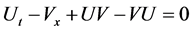 , we get the JM Equation (1.1).
We introduce a transformation
 (2.3)
(2.3)
with
 , (2.4)
 . (2.5)
The Lax pair (2.1) and (2.2) is transformed into a new Lax pair
 (2.6)
(2.6)
and
 (2.7)
(2.7)
We suppose that
 , (2.8)
where ,
,  ,
,  ,
,  ,
,  ,
,  are functions of
 ![]() and
and![]() .
.
Let ![]() and
and ![]() be two basic solutions of the Lax pair (2.1)
be two basic solutions of the Lax pair (2.1)
and (2.2). From (2.3), there exist constants ![]() such that
such that
![]() (2.9)
(2.9)
with
![]() (2.10)
(2.10)
There are ![]() Equations and
Equations and ![]() unknowns
unknowns![]() ,
, ![]() ,
, ![]() ,
, ![]() ,
, ![]() in (2.9). In order to determine these unknowns uniquely, we add another three Equations
in (2.9). In order to determine these unknowns uniquely, we add another three Equations
![]() (2.11)
(2.11)
The unknown ![]() in
in ![]() will be determined later.
will be determined later.
From (2.8) and (2.9), we have
![]() , (2.12)
, (2.12)
which means ![]() are roots of
are roots of ![]() (note that
(note that ![]() is independent of
is independent of![]() ).
).
Proposition 1. Let ![]() satisfy the Equation
satisfy the Equation
![]() (2.13)
(2.13)
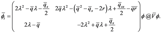
Through the transformation (2.3) with (2.4), the isospectral problem (2.1) is transformed into (2.6) with
![]() (2.14)
(2.14)
where ![]() are determined by (2.9) and (2.11).
are determined by (2.9) and (2.11).
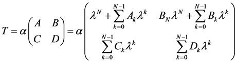
Proof. Let ![]() and
and
![]() , (2.15)
, (2.15)
It is easy to see that ![]() are (2N) th-order polynomials in
are (2N) th-order polynomials in![]() ,
, ![]() is a (2N-1)th-or- der polynomial in
is a (2N-1)th-or- der polynomial in![]() . By (2.1) and (2.10), we have Riccati Equation
. By (2.1) and (2.10), we have Riccati Equation
![]() . (2.16)
. (2.16)
Then all ![]() are roots of
are roots of![]() . Therefore we have
. Therefore we have
![]() , (2.17)
, (2.17)
where
![]()
and ![]() are independent of
are independent of![]() . We can rewrite (2.17) as
. We can rewrite (2.17) as
![]() (2.18)
(2.18)
By comparing the coefficients of![]() ,
, ![]() ,
, ![]() with (2.11) and (2.13), we get
with (2.11) and (2.13), we get
![]() : (2.19)
: (2.19)
![]() : (2.20)
: (2.20)
![]() (2.21)
(2.21)
![]() (2.22)
(2.22)
![]() : (2.23)
: (2.23)
![]() (2.24)
(2.24)
![]() (2.25)
(2.25)
From (2.21), (2.23) and (2.25), together with (2.11), (2.13), (2.14), (2.19), (2.20) and (2.24), we respectively get
![]() (2.26)
(2.26)
Comparing with (2.4) and (2.18), we find that![]() , and then
, and then ![]() and
and ![]() have the same form. □
have the same form. □
Remark. When![]() , supposing
, supposing![]() , DT is
, DT is
![]() (2.27)
(2.27)
Proposition 2. Let ![]() satisfy the Equation
satisfy the Equation
![]() (2.28)
(2.28)
where![]() ,
, ![]() ,
, ![]() are defined by (2.9) and (2.11),
are defined by (2.9) and (2.11), ![]() and
and ![]() are defined by (2.14). Through the transformation (2.3) with (2.5), the auxiliary spectral problem (2.2) is transformed into (2.7) with (2.14).
are defined by (2.14). Through the transformation (2.3) with (2.5), the auxiliary spectral problem (2.2) is transformed into (2.7) with (2.14).
To prove Proposition 2, we need to use Proposition 1 and the JM Equation (1.1), together with the help of the mathematical software (such as Mathematica). Although the idea of the proof for Proposition 2 is the same as Proposition 1, it is much more tedious and is omitted for brevity.
Since the transformation (2.3) with (2.14) transforms the Lax pair (2.1) and (2.2) into the same Lax pair (2.6) and (2.7), the transformation ![]() determined by (2.3) and (2.14) is called the DT of the Lax pair (2.1) and (2.2). Both the Lax pairs (2.1), (2.2) and (2.6), (2.7) obtain the JM Equation (1.1). Then, the transformation
determined by (2.3) and (2.14) is called the DT of the Lax pair (2.1) and (2.2). Both the Lax pairs (2.1), (2.2) and (2.6), (2.7) obtain the JM Equation (1.1). Then, the transformation ![]() determined by (2.3) and (2.14) is also called the DT of the JM Equation (1.1).
determined by (2.3) and (2.14) is also called the DT of the JM Equation (1.1).
3. Exact Solutions
In this section, by using of the above obtained DT, we get new solutions of the JM Equation (1.1).
For simplicity, taking![]() , we get two basic solutions of the Lax pair (2.1) and (2.2)
, we get two basic solutions of the Lax pair (2.1) and (2.2)
![]() (3.1)
(3.1)
with![]() .
.
According to (2.10), we get
![]() . (3.2)
. (3.2)
In the following, we discuss the two cases ![]() and
and![]() .
.
1) For![]() , from (2.9) and (2.11 ), we have
, from (2.9) and (2.11 ), we have
![]() (3.3)
(3.3)
with![]() . Then the exact solution of the JM Equation (1.1) is
. Then the exact solution of the JM Equation (1.1) is
![]() (3.4)
(3.4)
with![]() . This solution is similar with the solution in [11] .
. This solution is similar with the solution in [11] .
As![]() , this is a solitary wave solution where
, this is a solitary wave solution where ![]() is a kink-type soliton and
is a kink-type soliton and ![]() is a bell-kink-type soliton, i.e. this soliton is composed of a bell-type wave and a kink-type wave (see Figure 1).
is a bell-kink-type soliton, i.e. this soliton is composed of a bell-type wave and a kink-type wave (see Figure 1).
2) For![]() , from (2.9) and (2.11), we have
, from (2.9) and (2.11), we have
![]() (3.5)
(3.5)
where
![]() (3.6)
(3.6)
with
![]() . (3.7)
. (3.7)
The exact solution of the JM Equation (1.1) is
![]() (3.8)
(3.8)
When the parameters are suitably chosen, the solution (3.8) describes the elastic-inelastic-interaction coexistence phenomenon, i.e. the elastic and fission interactions coexist at the same time (see Figure 2).
In Figure 3, we can clearly find the interactions of the solitons. The solution ![]() is a solitary wave solution, where five kink-type solitons fuse into three kink-type solitons, i.e. K2 kink-type soliton and K4 kink-type
is a solitary wave solution, where five kink-type solitons fuse into three kink-type solitons, i.e. K2 kink-type soliton and K4 kink-type
![]()
![]() (a) (b)
(a) (b)
Figure 2. Plots of the solitary wave solution of (3.8) with ![]()
soliton are head-on interactions (this is an elastic interaction), K1 kink-type soliton, K3 kink-type soliton and K5 kink-type soliton fuse into K135 kink-type soliton (this is a inelastic interaction). The solution ![]() is a solitary wave solution, which is the same as
is a solitary wave solution, which is the same as![]() , but the solitons are the bell-kink-type (see also Figure 3). This phenomenon has been described in the Whitham-Broer-Kaup shallow-water-wave model [16] . It seems to be new for the JM Equation.
, but the solitons are the bell-kink-type (see also Figure 3). This phenomenon has been described in the Whitham-Broer-Kaup shallow-water-wave model [16] . It seems to be new for the JM Equation.