Asset Prices, Nominal Rigidities, and Monetary Policy: Role of Price Indexation ()
1. Introduction
A paper by Carlstrom and Fuerst [1] shows that equilibrium indeterminacy arises if monetary policy responds to share prices in a standard sticky-price economy. An increase in inflation reduces firm’s profits, and the share prices decline, since they reflect the firm’s profits. Then, the monetary policy response to share prices implicitly weakens overall reactions to inflation. This is a source of equilibrium indeterminacy.
In this paper, we extend the model of [1] by introducing price indexation and show that equilibrium determinacy is likely to arise. Under price indexation, the New Keynesian Philips curve is hybrid and has a lagged inflation term. It is shown that the effect of an increase in inflation on real marginal costs is weakened through the hybrid Phillips curve. Moreover, equilibrium indeterminacy caused by the monetary policy response to share prices never arises if all the firms that cannot re-optimize their prices follow price indexation.
An increase in inflation increases the real marginal cost under the sticky-price setting without price indexation, since a fraction of firms cannot change their prices. This increase in the real marginal cost implies low share prices. Then, the monetary policy response to share prices implicitly weakens overall reactions to inflation. Contrary to this, firms following price indexation can keep their real marginal cost constant in the long run since the past inflation reflects this increase in inflation.
[2] emphasize the inflation persistence by empirical analyses, and [3] develop a model with the hybrid New Keynesian Phillips curve. Many state-of-the-art DSGE models a la [4-6] employ price indexation. Therefore, it is important to consider the type of New Keynesian Phillips curve used when we investigate the relationship between monetary policy and share prices.
The rest of this paper is organized as follows. Section 2 introduces our model. Section 3 presents the main results and their interpretation. Finally, Section 4 presents our concluding remarks.
2. The Model
We employ a standard sticky-price model with shares, like [1]. The difference between our model and theirs is that we introduce price indexation in sticky prices.
2.1. Households
The household begins period t with 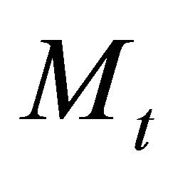 cash balances,
  one-period nominal bonds that pay
  gross riskfree interest rate,
  shares of stock that sell at price
 .
.
The utility function is
 (1)
(1)
where  is increasing in and concave,
  denotes consumption,
  denotes labor supply,
  denotes aggregate price level, and
  denotes real cash balances at the end of period t. The budget constraint of household is
 (2)
(2)
where 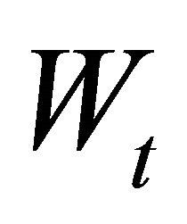 denotes wage rate,
 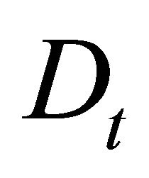 denotes dividends of share, and
  denotes monetary injection.
The first order conditions of households are

where  denotes gross inflation. The first equation is the intratemporal optimization condition, the second is the Euler equation for consumption, and the last is the Euler equation for share. The last equation can be rewritten as familiar asset prices equations:
 (3)
(3)
2.2. Firms
There are competitive final-goods firms and monopolistically competitive intermediate-goods firms and.
The production technology of final-goods firms is
 , (4)
, (4)
where  denotes the elasticity of substitution and
  denotes outputs of intermediate-goods indexed by i. The profit maximization of final-goods firms implies the demand curve for
  as
as
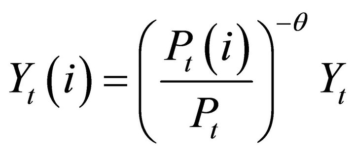 , (5)
, (5)
where  denotes the price level of intermediategoods indexed by i. Combining Equations (4) and (5) yields the following price index for intermediate goods:
 , (6)
, (6)
The intermediate-goods firms are monopolistically competitive, and they produce intermediate-goods 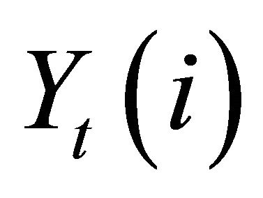 employing labor
 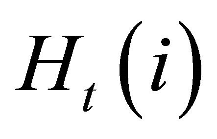 from households. The production function of intermediate-goods firm is
 , (7)
, (7)
The cost minimization problem implies
 (8)
(8)
where 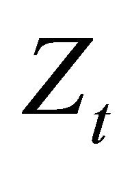 denotes the Lagrange multiplier of the cost minimization problem, and it can be interpreted as the real marginal cost.
Intermediate goods firms set their prices subject to Calvo-type price staggeredness with price indexation.
The price can be re-optimized at period t only with probability . Among
  firms that cannot reoptimize their prices, a fraction
  firms index their prices to the past inflation
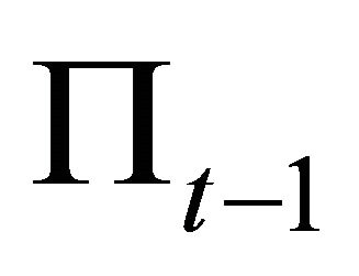 . As in [5,6], under this setting, we obtain the hybrid New Keynesian Phillips curve,
 (9)
(9)
where .
.  and
and 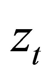 denote the log deviations from a steady state of inflation and the real marginal cost, respectively.
2.3. Monetary Policy
We assume that monetary authority follows a Taylor rule:
 (10)
(10)
where  and
and  denote the log-deviations from a steady state of
  and
and , respectively. If
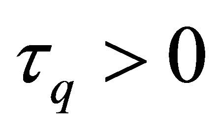 , a central bank responds to asset price fluctuations.
2.4. Equilibrium
The market clearing conditions are
 (11)
(11)
 (12)
(12)
 (13)
(13)
The resource constraint is
 (14)
(14)
and the aggregate production function is
 (15)
(15)
where  is a measure of resource cost of price dispersion:
 (16)
(16)
In this paper, we ignore effects from the price dispersion for simplicity.
We focus on a equilibrium where all monopolistic competitive firms are symmetric in this paper.
The firm’s profits are paid out as dividends to the shareholders. For simplicity, we assume that the measure of firms is equal to the measure of households.
The dividend of intermediate-goods firms is given by
 (17)
(17)
By Equation (8), the dividend is written by
 (18)
(18)
2.5. Linearized System
The linearized system is given as follows:
 (19)
(19)
 (20)
(20)
 (21)
(21)
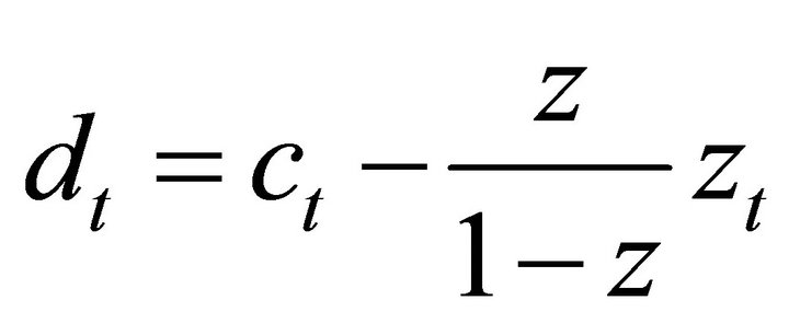 (22)
(22)
 (23)
(23)
 (24)
(24)
 (25)
(25)
where the lower letters denote the log-deviations from a steady state.
As shown by [1], the dividend is given by
 (26)
(26)
where

We employ an assumption on  following [1].
Assumption 1. .
.
Under this assumption, an increase in the real marginal cost decreases the dividend.
The equilibrium system is reduced to the following matrix form:

where

The first equation is the consumption Euler Equation (20); the second, the New Keynesian Phillips curve (24); and the third, the Euler equation for share (21).
In this paper, we impose the following restriction.
Assumption 2. .
.
We make this assumption to easily prove Proposition 1.
However, according to our numerical robustness check, the result in this paper is robust even if .
.
3. Main Results
3.1. Results
The main results of this paper are as follows.
Proposition 1. Under Assumptions 1 and 2 a necessary and sufficient condition for equilibrium determinacy is
 .
.
If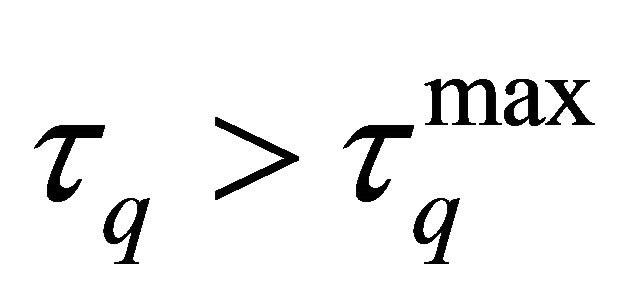 , there is equilibrium indeterminacy or no stationary equilibrium.
Proof. See Appendix Q.E.D.
At a limit of , the threshold
  is the same as the threshold in Proposition 1 of Carlstrom and Fuerst (2007).
The threshold  depends on the fraction of price indexation firms,
 .
.
Proposition 2.  is increasing in
 .
.
Proof. Since , we obtain
 Q.E.D.
Then, in the case where the fraction of price indexation is large, equilibrium determinacy is likely to arise even if monetary policy responds to share prices. Especially, in the case where , equilibrium indeterminacy never arises even if monetary policy responds to share prices.
Proposition 3. Under Assumptions 1 and 2, if all the firms follow price indexation,  , then equilibrium determinacy arises.
Proof. Q.E.D.
3.2. A Taylor Principle Interpretation
The Taylor principle establishes that a permanent increase in the inflation rate leads to a more-than-proportionate increase in the nominal interest rate. Following [1] and [7], we interpret our results according to this principle.
A one percentage point permanent increase in the inflation rate causes the marginal cost to increase by  percentage point through the New Keynesian Phillips curve. By the definition of
 , this can be rewritten as
 (27)
(27)
This decreases dividends and share prices by
 . The total effect on the nominal rate is given by
 (28)
(28)
If this total response is greater than unity, the rule satisfies the Taylor principle.
If , the coefficient of
  is strictly positive. Thus, monetary policy response to share prices weakens the total response to inflation and is a source of equilibrium indeterminacy. However, this effect is decreasing in
  since this coefficient of
  is decreasing in
 . This is because the effect of an increase in inflation on the real marginal cost, through the hybrid Phillips curve, is weakened. In particular, if
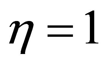 , then this coefficient is zero and the total effect on the nominal interest rate of inflation is
 . Therefore, monetary policy response to share prices is not a source of equilibrium indeterminacy in this case.
Under the sticky-price setting without price indexation, a fraction of firms cannot change their prices in every period. Then, a permanent increase in inflation implies a low real marginal cost. Under the sticky-price setting with price indexation, a fraction of firms that cannot re-optimize their prices indexes their prices to the past inflation. In the long run, firms following price indexation can keep their real marginal cost constant since the past inflation reflects this increase in inflation.
Therefore, a permanent increase in inflation does not change the real marginal cost if all the firms that cannot re-optimize their prices follow price indexation.
3.3. A Numerical Example
We have the fraction of firms that follow price indexation  affects the threshold of the central bank’s stance to the share prices on equilibrium indeterminacy qualitatively. In this subsection, we investigate the quantitative effects of
  on
on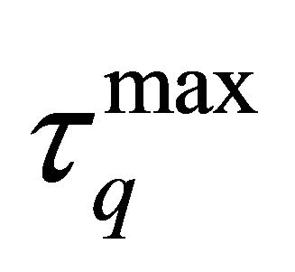 .
.
For this exercise, we set the parameter values of the model as follows. The discount factor of households,  , is 0.99. The relative risk aversion,
  , is two. The Frisch elasticity of labor,
  , is two. The central bank’s stance to inflation,
  is 1.5. The steady-state marginal cost,
  , is 0.85, which implies that the steady-state markup is 15%. These values are taken from those employed by [1]. We set the Calvo-pricing price-stickiness parameter,
  , is 0.75 following the literature, which implies that firms can re-optimize their prices about once a year.
Figure 1 shows the determinacy and indeterminacy regions. The vertical axis means the central bank’s stance to the share price. The horizontal axis means the fraction of firms that follow price indexation. The equilibrium indeterminacy arises in the upper-left region. The equilibrium determinacy arises in the lower-right region. Then, a stronger stance of the central bank to the share prices induces equilibrium indeterminacy. However, if the fraction of firms that follow price indexation is sufficiently high, equilibrium indeterminacy is not likely to arises if monetary policy responds to share prices.
4. Concluding Remarks
A recent paper by Carlstrom and Fuerst [1] found that monetary policy response to share prices is a source of equilibrium indeterminacy in a standard sticky-price model because an increase in inflation implies a high real marginal cost and low share prices.
In this paper, we investigated a sticky-price model in which the New Keynesian Phillips curve has a lagged inflation term caused by price indexation. We found that if firms follow price indexation, the effect of an increase in inflation on real marginal cost is weakened and equilibrium determinacy is likely to arise. Moreover, equilibrium indeterminacy never arises if all the firms that cannot re-optimize their prices follow price indexation.
Empirical results support the significance of a backward inflation term in the New Keynesian Phillips curve. Therefore, when we discuss the relationship between asset prices and monetary policy, we must consider the type of Phillips curve.
5. Acknowledgements
I would like to thank Timothy Fuerst, Masaru Inaba, and Keiichiro Kobayashi for their helpful comments and

Figure 1. Determinacy and indeterminacy regions.
suggestions. Of course, the remaining errors are mine. This work was funded by a Senshu University research grant (“Analyses of Monetary Policy Responses to Asset Price Fluctuations”) in 2011.
Appendix: Proof of Proposition 1
For equilibrium determinacy, just one root should be inside the unit circle and others should be outside the unit circle. It is easily shown that one root is . The three remaining roots are the solutions of a characteristic equation:

where

It is shown that , and
, and

since . A necessary condition for equilibrium determinacy is

In the case where all roots are real, it is obvious that this condition is also sufficient.
Next, consider the case where two roots are complex. Suppose that  are roots and a norm of
 . We have

where  is a real root in
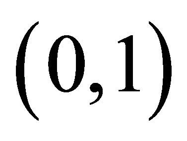 .
.
For equilibrium determinacy, we will show that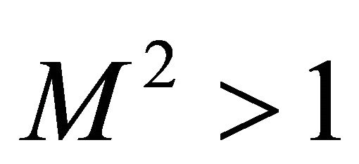 . By the form of
 , it is easily shown that
  reaches a local minimum at
 .
.
Since  and
and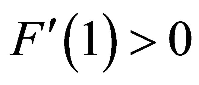 , it is shown that
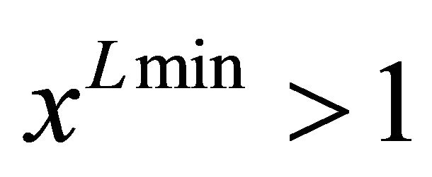 . It suffices to show that
  for for
 .
.
The rest of this proof, we show that 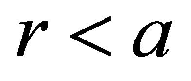 at first. Since
 , it is obtained that

If , we have

and it is a contradiction. Then, . Finally,
 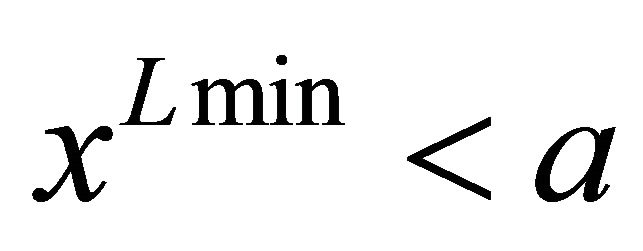 is shown as follows. A necessary and sufficient condition for
  is
is
 .
.
Since , this condition is reduced to

and this is easily shown.
Q.E.D.