Two-Dimensional Finite Element Method Analysis Effect of the Recombination Velocity at the Grain Boundaries on the Characteristics of a Polycrystalline Silicon Solar Cell ()
1. Introduction
To characterize solar cells, several studies, based for their majority on analytical methods, have been carried out in one dimension, two dimensions, or three dimensions [1] [2] [3] [4] [5] . These studies have permitted to characterize polycrystalline solar cells by determining the effects of the grain size and the recombination velocities for example, on the phenomenological and electrical parameters of the solar cell [1] [6] [7] [8] . The illumination level and the current-voltage characteristics were also studied [9] [10] . Unfortunately, each study required to carry out specific calculations according to the problem to be solved.
The objective of this study is to present a new approach of characterization of the solar cells, based on the finite element method. Using this method, the continuity equation in two dimensions can be solved, by modeling the crystal of a solar cell in 2D.
Compared to the analytical methods, in this approach, the results are obtained without redundancies of calculations for the various characteristics of the solar cell. In this study, we propose, for various values of the boundary recombination velocity Sgb, to determine the excess photogenereted carrier’s density, as well as the photocurrent density, the photovoltage and the current-voltage characteristics of the polycrystalline solar cell in the case where the thickness of the crystal solar cell is negligible comparatively to its width and its depth.
2. Theoretical Analysis
Let us consider a rectangular bifacial crystalline silicon solar cell having a base depth H1 and a width H2, illuminated successively on its front surface and on its back surface as represented in Figure 1.
One supposes moreover that no external electric or magnetic field is applied to the structure and the semiconductor substrate used is a thin layer, hence the effect of its thickness on the dynamics of the carriers is negligible.
In this case, the continuity equation which governs the solar cell’s operation is given by the following relation [1] :
 (1)
(1)
where  represents the photogenereted excess minority carrier’s density in the base, L, the diffusion length, D, the coefficient of diffusion and
 , the rate of generated carriers.
If this rate of generation depends only on x [1] , we have:
 (2)
(2)
The parameters ai and bi are the constants deduced from the modeling of the generation rate considered for the overall solar radiation spectrum [10] .
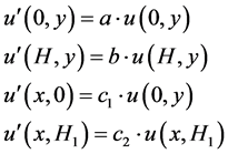
The continuity Equation (1) obeys to the following boundary conditions [1] , namely, the current of diffusion and the current of recombination are equal on the boundaries, i.e.:
- on the junction x = 0
 (3)
(3)
- on the back surface
 (4)
(4)
- on the y = 0 boundary
 (5)
(5)
- on the y = H2 boundary.
 (6)
(6)
Sj indicates the junction recombination velocity, Sb the back surface recombination velocity, and Sgb, boundary recombination velocity on the boundaries y = 0 and y = H2.
This continuity equation is an elliptic differential equation with Neumann boundaries conditions [11] . It can be written to the following general form:
 (7)
(7)
The associated Neumann’s boundary conditions are:
 (8)
(8)
where ,
,  ,
,  and
and .
.
2.1. Variational Formulation and Discretization of the Equation
The variational form associated with Equation (7) is:
 (9)
(9)
where , is the normal unit vector on the border
  and
and![]() , a normal deriva-
, a normal deriva-
tive on this border. To solve Equation (9), one subdivides the domain ![]() delimited by x = 0 and x = H1 according to Ox and y = 0 y = H2 according to Oy, into
delimited by x = 0 and x = H1 according to Ox and y = 0 y = H2 according to Oy, into
![]() triangular finite elements where N1 and N2 are positive integers. One has
triangular finite elements where N1 and N2 are positive integers. One has ![]() points for the mesh, as represented in Figure 2(a).
points for the mesh, as represented in Figure 2(a).
Let us consider a triangular finite element e and its three vertices 1, 2 and 3 with their respective coordinates (x1, y1), (x2, y2) and (x3, y3), as shown in Figure 2(b).
In this element e, ![]() can be approximated by a continuous solution
can be approximated by a continuous solution ![]() hence the approximate solution on whole domain
hence the approximate solution on whole domain ![]() is given by [12] .
is given by [12] .
![]()
m being the number of triangular finite elements of discretization.
For triangular finite elements, ![]() can be seeking in the linear form:
can be seeking in the linear form:
![]() (10)
(10)
After eliminating the constants a, b and c in above Equation (10), one obtains the carrier’s density of finite element e as follows:
![]() (11)
(11)
where ![]() indicate the values of carrier’s density at the vertices (1, 2, 3) and
indicate the values of carrier’s density at the vertices (1, 2, 3) and ![]() the coefficients given by:
the coefficients given by:
![]() (12)
(12)
![]() is the surface of triangular element such as:
is the surface of triangular element such as:
![]() .
.
![]()
Figure 2. (a) Two-dimensional discretization of the solar cell crystal, (b) tri- angular finite element e.
In each element, if one chooses ![]() as a trial function, these expressions of
as a trial function, these expressions of ![]() and
and ![]() introduced in the Equation (9) leads to the relation:
introduced in the Equation (9) leads to the relation:
![]() (13)
(13)
where ![]() and
and![]() .
.
The elements of the matrix ![]() (Stiffness matrix) are given for each triangular element by the integral [12] :
(Stiffness matrix) are given for each triangular element by the integral [12] :
![]() (14)
(14)
Those of the mass matrix ![]() are determined by:
are determined by:
![]() (15)
(15)
The elements of the matrix![]() , taking account of the boundary conditions and the orientation of the normal vector
, taking account of the boundary conditions and the orientation of the normal vector![]() , on the borders, are given by:
, on the borders, are given by:
![]() (16)
(16)
![]() (17)
(17)
![]() is a column matrix representing the second member. Its elements are given by:
is a column matrix representing the second member. Its elements are given by:
![]() (18)
(18)
Taking into account the contribution of each triangular element, one obtains the carriers density U to each node of the mesh after assembling all of the matrices ![]() and et
and et![]() . Thus this carrier’s density, after minimization of the variational form (9), obeys to the equation:
. Thus this carrier’s density, after minimization of the variational form (9), obeys to the equation:
![]() (19)
(19)
or inversely:
![]() (20)
(20)
A and L are the global matrix of Equation (13). The vector ![]() is the unknown excess minority carrier’s density.
is the unknown excess minority carrier’s density.
2.2. Current-Voltage Characteristics of the Solar Cell
By considering that the minority carriers flow in y-direction is weak compared to that in x-direction, the current-voltage characteristic of the solar cell is obtained by determining the photocurrent density J and the photovolatge V calculated from the relations (21) and (22) respectively as follow [1] [3] :
![]() (21)
(21)
q indicates the electron’s charge and
![]() (22)
(22)
![]() , represents the thermal voltage, Nb: the doping in the base,
, represents the thermal voltage, Nb: the doping in the base, ![]() , the intrinsic carrier’s concentration.
, the intrinsic carrier’s concentration.
3. Results and Discussions
3.1. Convergence Study
Using a numerical code that we conceived from this theoretical approach based on the finite element method, we have solved the continuity equation and analyzed the effects of recombination velocity at the grains boundary on the electric parameters of the solar cell. To validate our results, we initially determined the number of finite elements of the grid beyond that the solution converges. Thus, we have plotted in Figure 3, the minority carriers density photogenerated at the y = 0 plane boundary, for various values of the number of finite elements with![]() .
.
These curves shows that the convergence of the solution is obtained when N ≥ 30 i.e. for 1682 finite elements and 900 points of the mesh.
To ensure a good compromise between the precision and the computing time, we chose to use N = 30 finite elements.
3.2. Minority Carrier’s Density
We represented in Figure 4 and Figure 5, the excess minority carriers density according to base depth x, and the grain width y, when the solar cell is respectively illumination on its front surface and its back surface.
One notes that for the front surface illumination, the carriers density increases according to x, reaches its maximum around x = 0.175 mm, then it decreases and cancels when x = 0.3 mm. As for illumination on the back surface of the solar cell, the curve
![]()
Figure 3. Minority carrier’s density to the plane y = 0 boundary, for various values of N with D = 26 cm2/s, L = 0.01 cm, Sj = 106 cm/s, Sb = 105 cm/s, Sgb = 102 cm/s.
![]()
Figure 4. Minority carrier’s density, front surface illumination: D = 26 cm2/s; L = 0.01 cm; Sj = 106 cm/s; Sb= 105 cm/s; Sgb = 102 cm/s.
![]()
Figure 5. Minority carrier’s density, back surface illumination: D = 26 cm2/s; L = 0.01 cm; Sj = 106 cm/s; Sb = 105 cm/s; Sgb = 102 cm/s.
preserves the same profile but the maximum is reached around x = 0.25 mm.
We can also note a slight variation of these densities according to y, for both illuminations.
The effect of grain boundary recombination velocity on the minority carrier’s density is highlighted in Figures 6-9.
The grain boundary recombination velocity Sgb, reveals the carriers losses by recombination, at the grains boundaries. These losses significantly influence the profile of the
![]()
Figure 6. Minority carrier’s density, front surface illumination: D = 26 cm2/s; L = 0.01 cm; Sj =106 cm/s; Sb = 105 cm/s; Sgb = 0.
![]()
Figure 7. Minority carriers density front surface illumination: D = 26 cm2/s; L = 0.01 cm; Sj = 106 cm/s; Sb = 105 cm/s; Sbg = 103 cm/s.
excess minority carriers density as shown in these figures, represented according to the base depth and the grain width, respectively for Sgb = 0, Sgb = 103 cm/s, Sgb = 104 cm/s and Sgb = 106 cm/s. Sj and Sb being fixed at 106 cm/s and 105 cm/s.
![]()
Figure 8. Minority carriers density front surface illumination: D = 26 cm2/s; L = 0.01 cm; Sj = 106 cm/s; Sb = 105 cm/s; Sgb = 104 cm/s.
![]()
Figure 9. Minority carriers density front surface illumination: D = 26 cm2/s; L = 0.01 cm; Sj = 106 cm/s; Sb = 105 cm/s; Sbg = 106 cm/s.
When Sbg = 0, there are no losses by recombination at the grains boundaries. The photogenerated carrier’s density is more important. When Sgb increases, the recombination becomes more important and the carrier’s density decreases. We can note that at the grains boundaries (borders y = 0 and y = H2), the carriers density is weak. That is more and more remarkable when Sgb increases [1] .
When Sbg reaches the value of Sj = 106 cm/s, the carriers density becomes null at the boundaries.
Figure 10 and Figure 11 below represent the photogenereted minority carriers densities according to the base depth, with a boundary recombination velocity Sgb = 105 cm/s, and the junction recombination velocity Sj, respectively equal to 104 cm/s and 105 cm/s. The effects of Sj are definitely observable on these curves. That permits us to note the
![]()
Figure 10. Minority carriers density front surface illumination: D = 26 cm2/s; L = 0.01 cm; Sj = 104 cm/s; Sb = 105 cm/s; Sbg = 105 cm/s.
![]()
Figure 11. Minority carriers density front surface illumination: D = 26 cm2/s; L = 0.01 cm; Sj = 104 cm/s; Sb = 105 cm/s; Sbg = 105 cm/s.
widening of the space charge region ZCE and the reduction, even the cancellation of the carriers density at y = 0 and y = H2 planes boundary. These profiles of the carrier’s density permit to highlight the recombination phenomenon which is an important one in the solar cells operation [10] .
The same effects are observed when the solar cell is illuminated on the back surface as illustrated in Figure 12 for the same value of Sbg = 105 cm/s.
3.3. Photocurrent Density
The photocurrent density is determined starting from Equation (21). We have repre- sented it in Figure 13, versus the junction recombination velocity Sj, for various values of Sgb.
As waited, when Sj is equal to zero, the photocurrent density is null. When the junction recombination velocity Sj increases, the photocurrent density increases and is saturated when Sj reaches a critical value, corresponding to the short-circuit operation of the solar cell.
When the junction recombination velocity Sj is close to zero, the photocurrent density is null. That corresponds to the open-circuit operation of the solar cell. While when Sj is very large, the photocurrent density is constant and equal to the short-circuit current. We can also note that the open circuit or the short-circuit operation depends to the boundary recombination velocity Sgb. That is due to the fact that when Sgb is higher, losses by recombination are important.
3.4. Photovoltage
The photovoltage is one of the characteristic elements of the solar cell. Using our numerical code, we have determined the photovoltage and represented it in Figure 14,
![]()
Figure 12. Minority carriers density back surface illumination: D = 26 cm2/s; L = 0.01 cm; N = 30; Sj = 106 cm/s; Sb = 105 cm/s; Sgb = 105 cm/s.
![]()
Figure 13. Photocurrent density, front surface illumination; effect to Sbg: D = 26 cm2/s; L = 0.01 cm; Sb = 102 cm/s.
![]()
Figure 14. Photo tension front surface illumination: D = 26 cm2/s; L = 0.01 cm; Sb =105 cm/s.
according to the junction recombination velocity for various values of Sgb. This figure shows that when the junction recombination velocity Sj is close to zero, the photovoltage is equal to the circuit-open photovoltage Vco. and when Sj increases from zero to approximately Sj = 102 cm/s, the photovoltage remains constant and equal to the open circuit photovoltage. Beyond that value, the photovoltage decreases and cancels out when Sj reaches the short-circuit operation, for a value of Sj approximately equal to 1012 cm/s. We can also note that the open circuit photovoltage is larger when Sgb is smaller.
3.5. Current-Voltage Characteristics
The knowledge of the current-voltage characteristic is very important for the solar cell characterization. Using our code of calculations, we have determined and represented in Figure 15, the current-voltage characteristics of the solar cell for various values of the grain boundaries recombination velocity Sgb.
As awaited, these characteristics are in conformity with the solar cell operation. Indeed, one notes that when the photovoltage is equal to zero, the photocurrent density is equal to the short-circuit photocurrent density Jcc. When the photovoltage increases, the photocurrent density decreases and cancels, when the photovoltage reaches the open circuit photovoltage Vco.
One can notice that the open circuit photovoltage Vco and the short-circuit photocurrent density Jcc decrease when the grains boundaries recombination velocity Sgb increases [1] .
4. Conclusions
In this study we have realized a characterization of a polycrystalline silicon solar cell by the finite element method in 2D, by highlighting the effects of grains boundaries recombination velocity, on the electrical parameters of the solar cell.
From this new approach, the polycrystalline solar cell has been modelled and the photogenered excess minority carrier’s density has been determined. The characteristics of the solar cell (photocurrent density, photovoltage, and current-voltage) have been determined for various values of Sgb, highlighting the effects of the recombination at the grains boundaries on the solar cells operation.
![]()
Figure 15. Current-voltage characteristics of the solar cell for various values of Sgb, front surface illumination.
This approach based on a completely numerical method, permits to circumvent certain difficulties in the seeking of the solutions of equations which govern the solar cells operation.