Received 29 June 2016; accepted 25 July 2016; published 29 July 2016

1. Introduction
Previously in several papers [1] [2] by the author there was presented the mathematical model of turbulent fluid motion. In the model, a continuous medium (liquid, gas, etc.) is represented as an ensemble of discrete (liquid) objects. In general, depending on what is the meaning of the “discrete object” concept, generally speaking we can construct a set of mathematical models of turbulence [3] [4] . Semantic capacity of a discrete object concept is expressed, in particular, in a large number of synonyms used, such as liquid particles, mole, vortex, globule of the continuum, etc.
In the previously constructed model from the equations of inviscid incompressible fluid, it was deduced the potential used as an interaction potential between individual marked points of a continuous medium. The presence of the mathematical feature of the branching type is showed by the study of this potential in the framework of the two-body problem. This feature was considered as one of the most important characteristics of the turbulence phenomenon.
Presented in this paper, mathematical model of the motion of a perfect fluid is constructed from such point of view, when individual marked points of fluid are loaded with a weight and turn into discrete liquid particles. After specification of the mechanism of interaction of fluid pair particles model takes complete features and, in particular, allows performing a set of computational experiments on modeling different kinds of various flows. At all stages of constructing this model the effects associated with viscosity and thermal conductivity, are not taken into account. For this reason, this model is presented as a discrete model of a perfect fluid.
Overall, the model constructed below allowed us to separate deterministic and stochastic components in the description of turbulent flows of an ideal fluid. This separation is provided on an analytical level access to the mechanism of generation of stochastics and, consequently, to the possibility of constructing a typical representatives of the various classes of flows.
Note that the stochastic component in the dynamics of liquid particles in this model is a consequence of their interaction with each other and reflects the presence of the branching mechanism, previously studied on the example of the description of the dynamics of pairs of marked points of liquid. This type of stochastic is different, for example, from the stochastics specific for the class of lattice models of the Boltzmann equation (Lattice Boltzmann Method), used to describe the hydrodynamic flows [5] .
There is the well known method of direct numerical simulation of turbulent flows by solving the Navier- Stokes equations [6] [7] . This method generally is unstable due to the instability of flows with supercritical Reynolds numbers. In this case, the parameterization of stochastic component would allow to build any number of implementations of the given flow and to find all the necessary statistical characteristics. Because the liquid in the model is represented in the form of a set of identical liquid particles, so far this model has some common features with the models of granular media in terms of advances descriptions of these environments with liquid [8] [9] .
Various possible interpretations of a discrete object of a turbulent fluid can be divided into two groups. The first of these will take the submission of the discrete object as a particle. In this case, a particle refers to an object that is defined in the sense of classical mechanics, i.e. it has a fixed mass, position in space, velocity, etc. The second group will take the representation of the discrete object in the form of a wave. Under the wave is understood generally a geometrical structure through which the mass, energy, and other physical parameters flow. As an example, the representative of the second group is a vortex. The division into two groups in the interpretation of discrete liquid object is conditional, because in fact due to the turbulent mixing is not possible to draw a clear distinction between them. Thereby, the discrete object will be interpreted as both particle and wave, i.e. within the framework of a kind of “wave-particle” or “wave-corpuscle” dualism.
We note a number of works in the field of computational fluid dynamics, which may be interpreted from the standpoint of wave-particle duality. In the works of S. Ulam and coauthors [10] [11] discrete object is interpreted as a kind of “globule of continuum”. In the method of F. Harlow “particles in the cell” [12] and in the method of large particles [13] the cell can be regarded as standing waves, through which is flowing the stream of particles. Note that in the development of mixed Lagrangian-Eulerian numerical schemes for the calculation of currents [14] - [16] the main difficulty stems from the uncertainty the “corpuscular-wave” type in the interpretation of discrete object.
In general, the Eulerian and Lagrangian approaches of the continuous medium description are illustrative in connection with the dualism of particles and waves. For example, in the Eulerian approach being in a fixed point in space, the observer monitors the motion of the fluid that expressly assumes the wave interpretation of the cell in which it is located. In the Lagrange approach observer is located on the moving fluid, i.e. follows the movement of fixed particle. In the theoretical hydrodynamics Euler and Lagrange approaches are considered equivalent, but in practice the Euler approach prevails. Such preference Euler approach is due to the fact that in the Lagrangian approach for turbulent mixing to determine the particle it is impossible once and for all.
In this article considered in detail two-dimensional, the most studied case. Managed to build and explore using the computational experiment a number of interesting flows. Some regimes that provide separation of the particles in the ensemble were detected. Different kinds of vortex flows were simulated. Some interesting statistical properties of certain flows were detected. The flows, in which there is a concentration of kinetic energy in a small number of particles of the ensemble were detected. Discovered and studied also the flows, in which the kinetic energy of the particles is calibrated. In addition, it was possible using the appropriate flows of liquid particles of the ensemble to demonstrate the possibility to reproduce any prescribed image by manipulating the parameters of the interaction.
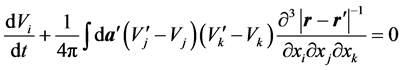
Briefly recall the procedure of entering into the consideration a discrete liquid particle under the model of turbulence developed earlier by the author. Write the equations of inviscid incompressible fluid:
 (1)
(1)
where i, j = 1, 2, 3; t―time, r = (x1, x2, x3)―radius-vector, v = v (t, r), P = P (t, r)―the velocity and the pressure fields, r = const > 0―density of the fluid (on repeated indices is implied summation).
Applies to the second equation in (1) the operation ¶/¶xi and take into account the condition of continuity, then
 (2)
(2)
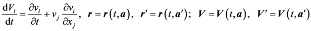
Formally, using the Green’s function, invert in (2) the Laplace operator. Performing twice the integration by parts assuming no motion at infinity and differentiating the resulting expression with respect to xi after some transformations and substitution in (1), we find

where v¢ = v(t, r¢), dr¢―element of volume in r¢-space.
At the Lagrangian approach in the description of the liquid is introduced vector function r = r (t, a), which represents the trajectory of the point with index . Velocity of point a is
  . The continuity implies that the Jacobian of the transformation
  does not depend on time. Choosing m = 1, and using the definition of V, we obtain
 (3)
(3)
where
We will approximate the integral in (3) in the sum by breaking the area of integration for simplicity on the same small amounts w, then
 (4)
(4)
where g =w /4p; n, m―numbers of small volumes w.
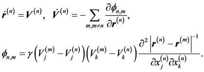
Thus, using the hypothesis of a discrete structure of turbulent fluid, reduce the study of the integro-differential Equation (3) to a system of ordinary differential Equation (4). At this stage, under the discrete object we will understand a point. Rewrite the system of Equation (4), introducing a binary interaction potential fn,m of the pair of points with numbers n and m:
 (5)
(5)
Suppose that for discretization of the space of initial conditions the fluid motion is approximated not by the motion of points, but by the motion of particles, then the following difficulty arises in the interpretation. The presence of turbulent mixing, as is known, leads ultimately to the fact that the particle, initially well defined in the context of the ensemble of particles will eventually fill the whole of the observed region of space. Thus, the particle’s individuality will be completely “erased” and it as though will “dissolve” into other particles. This is one of the main reasons why the equations of continuous medium in the form of Lagrange are so difficult to use in practice. That is why discrete objects at the level of Equation (5) are interpreted as points because it is natural to assume that the point remains the point throughout the time of movement.
Equation (5) were “prepared” in the form of a dynamic system the behavior of which is described by a set of radius vectors r(n) and the velocity V(n). The potential fn,m was first obtained in [17] . In our case, the potential is obtained by other means with an emphasis on the hypothesis of a discrete structure of turbulent fluid.
In the next section, we investigate the problem of motion of a pair of points. After that the points will be “loaded” weight and become more similar to liquid particles.
2. Investigation of the Interaction Potential
We rewrite (5), denoting by r1, r2; v1, v2―the radius and velocity vectors of a pair of fixed points of the liquid, then
 (6)
(6)
where v12 = v1 - v2, r12 = r1 - r2.
The system of Equation (6) has an integral of motion: v1 + v2 = const, which can be regarded as an analogue of the total momentum of the system. The existence of this integral fully characterizes the movement of the pair of points as a whole in the form of a rectilinear and uniform motion.
Let us turn to the study of the relative motion of a pair of points. For this purpose we introduce the notation r = r12, v = v12 and after the obvious manipulation in (6) we find
 (7)
(7)
By a direct calculation one can verify that the system of Equation (7) allows the following integrals of motion:

where
The integrals K and E can be considered as analogues of the conservation laws of angular momentum and energy. Going over to the coordinate system in which the vector K is directed along the axis x3, then the vectors r and v are in the plane of the variables x1, x2. We introduce in plane polar coordinates for the vectors r and v according to Figure 1. In this case, x1 = rcosa, x2 = rsina; v1 = vcosb, v2 = vsinb, then (7) reduces to the following system of equations:
 (8)
(8)
where y =b - a, while
![]()
The system of Equation (8) can be reduced to a pair of equations
![]() (9)
(9)
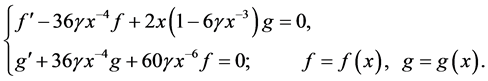
where y = ctgy. Dividing the first equation in (9) to the second one and introducing the dimensionless distance x = g-1/3r, we obtain
![]() (10)
(10)
Equation (10) has been numerically investigated earlier [18] . Figure 2 shows the resulting estimates of the numerical solution of Equation (10), for a set of solutions obtained when starting with the initial data taken from![]() . In this area, special lines x = 0 and y = 0 are allocated, and solutions by x are in the range of
. In this area, special lines x = 0 and y = 0 are allocated, and solutions by x are in the range of![]() , and by y in the range [?1; +1]. Point x = 61/3, y = 0 is a singular―saddle.
, and by y in the range [?1; +1]. Point x = 61/3, y = 0 is a singular―saddle.
In Figure 2 depicts three specific points: A1 = (0, 1/2), A2 = (0, -1/2) and the singular point of the saddle type C = (61/3, 0). The dashed lines in Figure 2 denote separatrices of the saddle which separates from each other the three types of trajectories. Conventional spans of points relative to each other with little or no interaction (trajectory area within the contour C1CC2). The movements, in which the point of flying from infinity, fall on a common center (the area below the contourA2CC2), and the movement symmetrical to them when the point splits into a pair of points, scattered to infinity (the area above the loop A1CC1). Finally, trajectories within the contour A1CA2 describe motion for the pair of points never flies apart at infinity.
The term “quasipair” was introduced in previous papers to designate to a pair of points that in the process of interaction fall to a common center, and stick together. It can be shown that the formation and decay of quasipair
![]()
Figure 1. Joint positioning vectors K, r and v.
![]()
Figure 2. Numerical solution of the Equation (10).
take place in a finite time, and from its formation to the breakup it “remembers” on integrals of motion K and E. This can be seen by studying the second Equation (9) in the neighborhood of a singular point A2, then, assuming
that y ® ?1/2, find, ![]() , K > 0. For the decomposition of the solution in a neighborhood of r = 0
, K > 0. For the decomposition of the solution in a neighborhood of r = 0
in terms of time, we can make a change of variables ![]() in the equation, after which it becomes clear that
in the equation, after which it becomes clear that ![]() at t®tf, where tf―the final time at which the distance between two points becomes zero.
at t®tf, where tf―the final time at which the distance between two points becomes zero.
Let us consider the process of disintegration of the quasipair. Assume that it is formed by moving the pair of points in accordance with one of the trajectories belonging A2 (Figure 2). In this case, it may be infinitely long and remain in that state with y = ?1/2. If we assume that a transition y from the value of ?1/2 to +1/2 (the integrals of motion does not change), the quasipair starts to disintegrate under the symmetric trajectory, emerging from the A1.
In the vicinity of r = 0, i.e., at the time of the fall (decay) of the points to each (from) other, according to (8), we have![]() . The last equation means that the angular velocity
. The last equation means that the angular velocity ![]() of the rotation of vector r increases without limit, or, in other words, the quasipair is a point vortex. It is clear that after the decay of the quasipair and of the dispersion of the points by some distance from each other, the direction of expansion can be arbitrary in the plane perpendicular to the vector K. The angle describing the direction of scattering can be selected as a parameter, which describes the set of permissible trajectories. Each trajectory from this set is no highlighted, so for the real description of the decay of quasipair it is necessary to postulate the existence of a mechanism describing the random equiprobable choice from the set of permissible trajectories.
of the rotation of vector r increases without limit, or, in other words, the quasipair is a point vortex. It is clear that after the decay of the quasipair and of the dispersion of the points by some distance from each other, the direction of expansion can be arbitrary in the plane perpendicular to the vector K. The angle describing the direction of scattering can be selected as a parameter, which describes the set of permissible trajectories. Each trajectory from this set is no highlighted, so for the real description of the decay of quasipair it is necessary to postulate the existence of a mechanism describing the random equiprobable choice from the set of permissible trajectories.
Thus, to describe the process of formation and decay of quasipair it is not enough Equation (7). It is necessary to define additionally two mechanisms: the transition of quasipair from state with y = ?1/2 to a state with y = +1/2 and equiprobable selecting of one of a set of the trajectories which are permitted to occur in the plane perpendicular to the vector K. Thus we can speak about the presence of the branching point singularity in Equation (7).
From the standpoint of the problem of describing of a pair of points motion, so formed quasipair can exist infinitely long due to the fact that any later date is not highlighted. The uncertainty in the lifetime of the quasipair will be eliminated with using the liquid particles ensemble constructed below.
Figure 3 shows a graphical image of the formation and decay of quasipair. A pair of points in accordance with the in-trajectory falls on a common center, visually it can be interpreted as the formation of a vortex. When a pair of points will fall on a common center, a quasipair will form that can continue to exist infinitely long. If allow it to decay, it can be implemented in accordance with the out-trajectory, an example of which is shown in Figure 3. Note that both (in and out) the trajectories are in a plane perpendicular to the momentum K.
The presence of branching in a system consisting of a pair of points, suggests that this phenomenon is typical for Equations (5), which describe the motion of an ensemble of points of the liquid. Now, a natural question arises. How to relate to each other the results of the study of the motion of an ensemble of points of the fluid with the original equations of inviscid incompressible fluid?
Note that the transition from continuous to discrete in the form in which it was done above leads to the fact that talk about the condition of continuity in a discrete aspect is meaningless. For this reason, the system of Equation (5) has only indirect relevance to nonviscous incompressible fluid equations. The transition to a discrete representation and the study of it from the point of view of the movement points of a liquid allows us to take a new look at the main hydrodynamic nonlinearity, i.e. quadratic in the velocity term in the equations of motion of a continuous medium. In this case, Equation (5) can be considered as a special tool that allows you to reveal the mechanism of branching, due to the quadratic in the velocity hydrodynamic nonlinearity.
It is interesting to compare our point of view with the position of the dynamic chaos [19] in the interpretation of the phenomenon of turbulence. As in the first and in the second case we can talk about the movement trajectories of some labeled points. In both approaches, there are moments of close convergence of the trajectories of a pair (or more) points. If in our model, this convergence ends with the actualization of the branch point, then in the model of dynamic chaos paths are dispersed exponentially. Branching suggest the “man-made” introduction
![]()
Figure 3. Graphic illustration of the formation and decay of quasipair.
of stochastics for resolution of the question of choosing a certain trajectory from the set of permissible ones. In this case, the stochastic mechanism is external with respect to the equations describing the motion of fluid points. In the model of dynamic chaos, in the strict sense, there is no stochasticity. In this case, the term “stochasticity” has the meaning, such as random choice from the set of feasible outcomes. In this regard, the following questions arise. Have generally any sense the branching themselves? Whether branching is a product of the inadequacy of our way of describing the continuum? It seems that the discovered mechanism of branching is an extreme form of manifestation of turbulence in the fluid motion representation logic describing the set of points movement.
3. Onwards to an Ensemble of Liquid Particles
In sections 1, 2, fluid flow was considered as a movement marked points. In this case, it was found that a pair of points can fall on each other over a finite time to form an intermediate point―quasipair. Quasipair after a certain period of time is divided into two points, and there are many ways of break up, satisfying the integrals of motion. Possible decay trajectories are characterized by the presence of features such as branching in the mechanism of formation and decay of quasipair.
Now put the following task. We will construct an ensemble of discrete liquid particles again using only a few necessary results mentioned in Sections 1, 2, in particular those related to the mechanism of formation and decay of quasipair. For this we will represent a liquid as a set of separate liquid particles. Following the analogy between turbulence and ordinary gas atoms, the liquid will be presented initially in the form of rarefied gas of liquid particles that move between collisions rectilinearly and uniformly. We assume that the chosen discrete liquid particles are of circular shape for two-dimensional case and the spherical form in three-dimensional space.
Let a pair of liquid particles moving closer to a distance equal to or less than the sum of their radii, then assume that the pair coalescence occurs with the formation of an intermediate particle, i.e. quasipair. The quasipair is a metastable object and after some time splits into a pair of liquid particles. Formation and decay of quasipair stepwise interprets the collision of a pair of liquid particles, in this case should be the laws of conservation of mass, momentum, energy and angular momentum.
We assume that the quasipair exists during the interaction of a pair of particles, i.e., quasipair is another name of the mechanism of interaction. By particle collisions, the size and weight of which, generally speaking, are unequal to each other, the quasipairs are formed, which then decays into a pairs of identical particles. The last condition is justified by the fact that quasipair has one preferred axis passing through its center along the angular momentum. Thus, if the original liquid was represented by a set of liquid particles with a corresponding distribution of volumes and masses, the further evolution of the system will lead to a state where the volumes and masses of the particles are the same. Hereinafter we assume that the masses of all liquid particles are equal and have the value of m. It should be noted that the decay of the quasipair into two identical liquid particles was previously interpreted by the author as an elementary act of turbulent mixing.
If we consider the mass of the particles as a marker of individuality then due to the mechanism of formation and decay of quasipair and mass redistribution between the particles, it follows that the individuality of particles is not saved―they constantly acquire new masses and lose old ones. In other words, they can be regarded as the objects of the wave nature. In the intervals between collisions, discrete objects may be considered as liquid particles, in the moment of collision and during the quasipair’s lifetime the wave nature of fluid particles is emerged. In this it manifests itself wave-particle duality of the discrete object, interpreted in this model as a liquid particle.
At first, we study an ensemble of two-dimensional liquid particles. Without loss of generality, we place an ensemble of particles into the region shape a square with a side of L. For simplicity, the square-shaped area we will call a box. We assume that the liquid particles are elastically reflected from the walls of the box. Figure 4 shows the positioning of the square box and a fluid particle which moves with constant velocity, elastically reflected from the walls.
Let us choose some size L of the original box. Fluid particle we will represent as a circle with a radius r0. Position of the particle will be characterized by the radius vector r = (x, y), where x and y―abscissa and ordinate of the center of the liquid particle in the form of a circle. The velocity of the particle will be denoted by the radius vector v = (vx, vy), where vx and vy―projections of the velocity vector v on the axis of abscissa and ordinate.
Let at some point of time t the position and the velocity of the liquid particle are r and v respectively. We
![]()
Figure 4. The movement of one liquid particle in a square box, L = 1.
define the time step t, and the position and velocity of the fluid particle in the time moment t + t and we denote by the symbols ![]() and
and ![]() respectively. In this case, if the future position of the particle is within a box, i.e.
respectively. In this case, if the future position of the particle is within a box, i.e. ![]() and
and ![]() then
then
![]() (11)
(11)
In the case where ![]() either
either![]() , then
, then
![]() (12)
(12)
In the case where ![]() either
either![]() , then
, then
![]() (13)
(13)
Conditions (11)-(13) provide the motion of the center of the liquid particle within the box, in this case the particle is elastically reflected from the walls. Figure 4 shows a selected portion of particle dynamics, where the current velocity of the particle is designated with the radius vector. For realization of a computational experiment on the modeling of fluid particle move according to the algorithm (11)-(13) it is necessary to impose a limitation on the time step t, namely![]() , where
, where![]() is the module of the liquid particle’s velocity.
is the module of the liquid particle’s velocity.
4. Interaction of a Pair of Discrete Liquid Particles
Let us consider in the area of the square form a pair of liquid particles, which interact with each other and with the walls of the box. Interaction with the walls describe according to the algorithm (11)-(13). Separately focus on describing the interaction of pair liquid particles.
Denote the current position and velocity of the particles before the interaction radius vectors r1, r2 and v1, v2, respectively. After the interaction, the position and velocity of particles is denoted the radius vectors ![]() and
and![]() .
.
Define the known in mechanics two pairs of variables r, R and v, V to describe the interaction of two particles of equal mass:
![]() (14)
(14)
The vector R defines the position of the center of mass of the pair of particles, and V―velocity vector of the center of mass. The vector r describes the relative radius vector of the position a pair of particles, and v―rel- ative velocity pair of the particle.
From (14) we can write the position and velocity of each of the particles through pair new variables:
![]() (15)
(15)
Let at the interaction of pair liquid particles the law of conservation of momentum is satisfied, then
![]() (16)
(16)
After substitution of the second pair of Equation (15) to the left and similarly to the right side of Equation (16), we obtain
![]() (17)
(17)
Ensure compliance with the law of conservation of energy, then
![]() (18)
(18)
After substitution of the second pair of Equation (15) to the left and similarly the right side of (18), we obtain
![]() (19)
(19)
Taking into account (17), we find
![]() (20)
(20)
where v = |v|, v¢ = |v¢|.
At last, we write the condition for the fulfillment of the law of conservation of angular momentum, i.e.
![]() (21)
(21)
Taking into account (15) Equation (21) can be rewritten as:
![]() (22)
(22)
In connection with the implementation of the law of conservation of angular momentum, we assume that the interaction does not change the position of the center of mass of the pair of fluid particles, i.e.
![]() (23)
(23)
Taking into account (17), (23) in (22), we find
![]() (24)
(24)
Let a and b the angular deviation of the vectors r and v from the x-axis. Analogously angles a¢ and ![]() we understand angular distance from the x-axis vectors r¢ and v¢. In this case, passing to the polar coordinate system, we can write:
we understand angular distance from the x-axis vectors r¢ and v¢. In this case, passing to the polar coordinate system, we can write:
![]()
![]()
where r = |r|, v = |v|; r¢ = |r¢|, v¢ = |v¢|.
Substituting the polar representation of the relative position and velocities in vector cross products (24), we find
![]() (25)
(25)
Along with the (24) we make another assumption about the mechanism of interaction in connection with the law of conservation of angular momentum, namely
![]() (26)
(26)
Assumptions (23) and (26) clarify the geometry of the interaction of a pair of fluid particles and may be considered as postulates.
We introduce notation for the relative angles between the radius vectors of positions and velocities: y = b ? a and![]() . After substituting (20) and (26) in the last equality (25) we find
. After substituting (20) and (26) in the last equality (25) we find
![]() (27)
(27)
Equation (27) has two classes of solutions:
1)![]() ; 2)
; 2)![]() (28)
(28)
where ![]()
Formulate a criterion of interaction of pair of liquid particles in the form both of the following two conditions:
![]() (29)
(29)
where (r, v)―scalar product of two vectors. According to the criterion (29), a pair of liquid particles interact under two conditions: firstly, the distance between the particles become less or equal to two radii of particles and, secondly, the projection of the relative speed on the relative distance is negative, i.e. centers of particles approach one another.
The criterion of interaction (29) can be rewritten as:
![]() (30)
(30)
Taking into account (30) let us assume that the interaction is terminated when condition
![]() (31)
(31)
is satisfied.
It is easy to see that condition (31) is satisfied on the second class of solutions (28). Indeed, since![]() , insofar cosy < 0, which is true by (30).
, insofar cosy < 0, which is true by (30).
Let us write![]() , then taking into account that cosy < 0, we find generally a couple solutions that
, then taking into account that cosy < 0, we find generally a couple solutions that
can be represented as:
![]() (32)
(32)
where![]() ,
, ![]() ,
,![]() . To determine n, we substitute (32) into the second equality in (25), then we find
. To determine n, we substitute (32) into the second equality in (25), then we find
![]() (33)
(33)
where sign(K)―signum-function of magnitude K.
Substituting (33) in the second class of solutions (28), we find
![]() (34)
(34)
Taking into account that![]() , rewrite the solution (34) in the form
, rewrite the solution (34) in the form
![]() (35)
(35)
Equations (34), (35) are the key issue in the study of the interaction of a pair of liquid particles. According to Equation (35) angular deviation from the abscissa a¢, ![]() radius vectors of the relative positions r¢ and velocities v¢ of a pair of liquid particles can be any of ones if they according to Equation (35).
radius vectors of the relative positions r¢ and velocities v¢ of a pair of liquid particles can be any of ones if they according to Equation (35).
As a consequence of Equation (35) occurs an additional freedom of choice of angles in each act of interaction of pair of particles. For example, suppose that in any way the angle a¢ is determined, then the angle ![]() can be found using (35). Conversely, if the angle
can be found using (35). Conversely, if the angle ![]() is defined, a¢ angle can be found by using (35).
is defined, a¢ angle can be found by using (35).
Figure 5 shows a graphical illustration of the interaction of a pair of liquid particles, when it is considered that a¢ = p/4 and![]() . The circles in Figure 5 indicate the interacting particles, with the dashed line indicating the particles after the interaction. More bold line of the circle denotes the particle №1, and less fatty―particle №2. Centers of the circles marked stars and pentagrams before and after the interaction.
. The circles in Figure 5 indicate the interacting particles, with the dashed line indicating the particles after the interaction. More bold line of the circle denotes the particle №1, and less fatty―particle №2. Centers of the circles marked stars and pentagrams before and after the interaction.
To complete the description of the mechanism of interaction of a pair of liquid particles it is necessary to supplement a new configuration of a pair of particles with criterion that it is fitted in the selected box.
Positions and velocities of particles in a moment of time t before and after the interaction denoted by the symbols: r1 = (x1, y1), r2 = (x2, y2), v1 = (v1,x, v1,y), v2 = (v2,x, v2,y) and![]() ,
, ![]() ,
, ![]() ,
,![]() . Symbol “^” will denote the position and velocity of particles at time t + t, where t is the time step.
. Symbol “^” will denote the position and velocity of particles at time t + t, where t is the time step.
If any of the new positions ![]() and
and ![]() of the particles after the interaction went beyond the selected box, then these positions are adjusted through a slight of the procedure of reflection. Clarify the procedure on the example of the first particle, the application of the procedure to the second particle is similar.
of the particles after the interaction went beyond the selected box, then these positions are adjusted through a slight of the procedure of reflection. Clarify the procedure on the example of the first particle, the application of the procedure to the second particle is similar.
The procedure includes the following checks and transformation: if![]() , then
, then![]() ,while, when
,while, when
![]() , then
, then![]() ; if
; if![]() , then
, then![]() , while, when
, while, when![]() , then
, then![]() ; if
; if![]() ,
,
then![]() , while, when
, while, when![]() , then
, then![]() ; if
; if![]() , then
, then![]() , while, when
, while, when
![]() , then
, then![]() . A similar procedure is applied after the interaction to the second particle. In all other
. A similar procedure is applied after the interaction to the second particle. In all other
![]()
Figure 5. The geometry of the of interaction of pair of liquid, when a¢ = π/4,![]() .
.
cases, it is considered that![]() .
.
As a result, we can formulate the following algorithm, which simulates the movement of the pair of liquid particles interacting with each other and with the walls of the box. Suppose that at time t the positions and velocities of particles are r1, r2 and v1, v2, respectively. Find at time t + t new positions ![]() of the particles according to the formulas:
of the particles according to the formulas:![]() ,
,![]() . We check out particles outside the box or not? If left, then return them to the boundaries of the box using the procedure (11)-(13). Further, check the satisfaction of the criterion of the interaction (29), (30). If the criterion is satisfied, find new positions of the pair of particles
. We check out particles outside the box or not? If left, then return them to the boundaries of the box using the procedure (11)-(13). Further, check the satisfaction of the criterion of the interaction (29), (30). If the criterion is satisfied, find new positions of the pair of particles![]() . We check their entrance into the original box and apply the procedure described above of particle return to the original area. After all these steps, we find the positions
. We check their entrance into the original box and apply the procedure described above of particle return to the original area. After all these steps, we find the positions ![]() and velocities
and velocities ![]() of the pair of particles at time t + t.
of the pair of particles at time t + t.
We introduce a second constraint along with the constraint![]() . To the dynamics itself in the form of a motion separate from each other liquid particles occurred it is necessary to assume that
. To the dynamics itself in the form of a motion separate from each other liquid particles occurred it is necessary to assume that![]() .
.
To complete the procedure of modeling the motion of a pair of particles in the area of the square form is necessary for each act of interaction between pairs of particles to clarify the option of angles a¢, ![]() , which must satisfy the condition (35).
, which must satisfy the condition (35).
Consider the example where the angle a¢ is chosen uniformly randomly from the interval [0, 2π]. Taking into account (35) we write
![]() (36)
(36)
where x―uniformly distributed on [0,1] random variable.
Figure 6 shows a graphic image of a fragment of the dynamics of a pair of interacting particles in a box of unit length and width, and the angular deviation of the radius vectors of relative positions and velocities of pair of particles were chosen according to the expression (36).
Let us examine with how many particles simultaneously interact with each other according to the criterion (29), (30). In Figure 7(a) is shown an example of a random arrangement of N = 200 particles in a box with sides L = 1. It is also believed that the particles in the box have uniformly random velocities coordinates in the interval [?Vmax, Vmax]. Pairs of particles that interact according to the criterion (29), (30) are indicated in Figure 7(a) by connecting the centers of the respective particles with the line. From Figure 7(a) is shown that, for the chosen values of the parameters, of individual pairs of interacting particles is quite a few.
![]()
Figure 6. Fragment of a dynamics of a pair of interacting particles, L = 1, r0 = 0.1.
![]() (a)
(a)![]() (b)
(b)
Figure 7. (a) The sample of a random arrangement of the particles in a box with random velocities, as well as a pair of interacting particles; (b) A plot of the number of binary relationships Nb on particle radius r0.
From geometrical considerations it is clear that with increasing fluid particle radius r0 the number of binary relationships with a random arrangement of positions and velocities must increase, while the single binary relationships will be less. In other words, the particles will interact with many other particles. According to Figure 7(a) we can talk about clusters. The clusters could be distinguished by the number of particles that are included in it, while, of course, clusters with the same number of particles may differ from each other in the configuration of set of binary relations.
Figure 7(b) shows a plot of the number of binary links Nb in the ensemble on the parameter r0, when r0®L. It is clear that the number of binary links cannot exceed the maximum possible number of N(N ? 1)/2. The value of this parameter is shown on Figure 7(b) as the upper dotted line. It was found that when r0®L and at a random location of the provisions of the particles, as well as random values of their velocities, the number of binary links is committed to half of the maximum possible number. Finally, in Figure 7(b) is shown the lower dashed line, which represents the maximum possible number of clusters consisting of two particles, the apparent number of which is N/2. Such clusters we call 2-clusters, referring to n clusters,![]() .
.
Let us study question about the number of 2-clusters. Denote the number of 2-clusters in the ensemble of the liquid particles through Cl2. The fraction of 2-clusters in the set of all binary relations we denote by S2. Under share 2-clusters refers to the ratio of the number of 2-clusters Cl2 to the total number of binary relations Nb, i.e.
![]() . Figure 8 shows the desired curves obtained using Monte Carlo computational experiment.
. Figure 8 shows the desired curves obtained using Monte Carlo computational experiment.
The curve on the left graph Figure 8 demonstrates a maximum, which is located in a neighborhood of the
relation![]() . The right graph Figure 8 shows the dependence of the fraction of 2-clusters on the radius
. The right graph Figure 8 shows the dependence of the fraction of 2-clusters on the radius
of the liquid particles. When ![]() an approximate fraction of 2-clusters in the total set of binary relations is 50%.
an approximate fraction of 2-clusters in the total set of binary relations is 50%.
5. Interaction in the n-Cluster
As in the study of the interaction of pairs of particles, we define the position R and the velocity V of the center of mass of some n-cluster, i.e.
![]()
Figure 8. Graphics of the number and proportion of 2-clusters from the radius of the liquid particles.
![]() (37)
(37)
where![]() ;
;![]() ―positions and velocities of n particles included in the n-cluster. For simplicity, the numbering of the particles in the cluster selected natural, i.e.
―positions and velocities of n particles included in the n-cluster. For simplicity, the numbering of the particles in the cluster selected natural, i.e.![]() , in the general case, however, this is the set of numbers
, in the general case, however, this is the set of numbers ![]() from the original list of numbers
from the original list of numbers ![]() of the ensemble of particles.
of the ensemble of particles.
A set of n particles takes the form n-cluster when any particle from the set ![]() interacts according to the criterion (29), (30) with at least one other particle of the same set. In other words, for each i-th particle (
interacts according to the criterion (29), (30) with at least one other particle of the same set. In other words, for each i-th particle (![]() ) there exists at least one j-th particle such that
) there exists at least one j-th particle such that
![]() (38)
(38)
where ri,j = ri ? rj, vi,j = vi ? vj.
Taking into account (37) we write a representation for the positions and velocities of the particles of n-cluster, namely
![]() (39)
(39)
where
![]() (40)
(40)
According to (40) it is easy to verify that![]() .
.
Let us consider the law of conservation of momentum in the n-cluster. In this case we assume that the equality of such form is true:
![]() (41)
(41)
where a dash will denote the corresponding characteristics of the particles after interaction in the n-cluster, i.e. ![]() are the velocities of the n-cluster particles after interaction.
are the velocities of the n-cluster particles after interaction.
Taking into account (37), (39), the law of conservation of momentum can be rewritten in the form:
![]() (42)
(42)
According to the law of conservation of momentum in the form of (42) velocity of the center of mass of the n-cluster after the interaction does not change.
Let us consider energy conservation law, more precisely the kinetic energy in the n-cluster, namely
![]() (43)
(43)
Substituting in (43) representation for the particle velocity from (39), we find
![]() (44)
(44)
According to the law of conservation of energy in the form of (44) the sum of squares of the velocities ![]() is saved after n-particle interaction in the cluster.
is saved after n-particle interaction in the cluster.
Let us consider law of conservation of angular momentum in the n-cluster. We write it as:
![]() (45)
(45)
where![]() ―the positions of the particles after the interaction in the n-cluster.
―the positions of the particles after the interaction in the n-cluster.
Substituting the representation (39) in (45), we find
![]() (46)
(46)
In connection with the law of conservation of angular momentum in the form of (46) will make a number of statements that can be considered as additional postulates concerning the mechanism of interaction in the n-cluster. We assume that after the interaction position of the center of mass of the cluster particles does not change, i.e.
![]() (47)
(47)
Taking into account (42), (47) in (46), we rewrite the condition of conservation of angular momentum in the form:
![]() (48)
(48)
At this stage, being limited two-dimensional case, we can write the following representation for the positions and velocities of the particles of n-cluster before and after the interaction:
![]() (49)
(49)
where![]() ―the angular deviation from the x-axis of the vectors qi, ui of the i-th particle before and after the interaction.
―the angular deviation from the x-axis of the vectors qi, ui of the i-th particle before and after the interaction.
Substituting in (48) presentation (49), we find
![]() (50)
(50)
where![]() .
.
Will have two statements regarding the mechanism of interaction in the n-cluster in connection with the implementation of the law of conservation of angular momentum, namely
![]() (51)
(51)
According to (51), it is believed that the modulus of distances and velocities relative to the center of mass of particles in n-cluster remain unchanged after the interaction. In particular, the second condition ensures that the law of conservation in the form of (44).
Taking into account (51), we rewrite Equation (50), then we find
![]() (52)
(52)
Equation (52) is the generalization to the n-cluster Equations (27), constructed for 2-cluster in connection with the implementation of the law of conservation of angular momentum.
Following (28), will choose as the solutions of Equation (52), the following two sets of values of the angles yi and![]() :
:
1)![]() , 2)
, 2)![]() (53)
(53)
where ![]()
To choose as one of the solutions in the two sets of (53), let us consider in more details the criterion of interaction (38) in terms of the sign of the scalar product![]() .
.
According to the criterion of interaction in the form (38), if a pair of particles interact, then![]() . Let us try to find the angles
. Let us try to find the angles ![]() so that after the interaction for all pairs of coupled particles condition
so that after the interaction for all pairs of coupled particles condition ![]() was just the opposite, i.e.
was just the opposite, i.e.![]() .
.
Taking into account (51) write the expression for the scalar product before and after the interaction, then
![]() (54)
(54)
![]() (55)
(55)
In addition to Equations (54), (55) it is still need to take into account the requirement that ![]() before and after the interaction, i.e.
before and after the interaction, i.e.
![]() (56)
(56)
In summary, we conclude that it is necessary to choose the angles ![]() so as to satisfy simultaneously the conditions (53)-(56). Direct check shows that the dependence of the form
so as to satisfy simultaneously the conditions (53)-(56). Direct check shows that the dependence of the form
![]() (57)
(57)
where![]() , m―arbitrary angle, allows simultaneous fulfillment of conditions (54)-(57). In particular, ac- cording to (57) it was found that a suitable class of solutions in the (53) is 2), because after subtracting the first equation from the second in (57) we find
, m―arbitrary angle, allows simultaneous fulfillment of conditions (54)-(57). In particular, ac- cording to (57) it was found that a suitable class of solutions in the (53) is 2), because after subtracting the first equation from the second in (57) we find![]() . Conditions (55), (56) with (57) are easily verified.
. Conditions (55), (56) with (57) are easily verified.
As a result, according to (54)-(57), succeeded to find such conditions under which an arbitrary n-cluster ceases to exist after the interaction. In other words, the binary relationships that ensure the existence of the n-cluster cease to exist after the interaction according to the scheme (54)-(57).
For example, consider the experiment of the formation and disappearance of 4-cluster with a special choice of the initial data. Suppose that from the four corners of the original box with the same velocities directed along the diagonals begin to move 4 identical particles. After some time, they are found in the center region, forming a 4-cluster. It is necessary to observe the further dynamics.
Figure 9 shows the three fragments of the dynamics at three points in time. In Figure 9(a) shows the configuration of four particles after the first time step (t = 0, 1). Vectors in Figure 9 show the particles velocities. In Figure 9(b) and Figure 9(c) the configurations of the particles before and after interaction at the 4-cluster are presented. In the interaction presented in Figure 9 described according to scheme (53)-(57), it was assumed that m = p/4.
After studying the interaction of particles in n-cluster has became clear a possible algorithm for calculation the dynamics of the ensemble. Let at some time t are found all the clusters which in general can be divided into 2-clusters, 3-cluster, ![]() , k-clusters. Each of the clusters can be represented as a set of their structural analogues in the amount of
, k-clusters. Each of the clusters can be represented as a set of their structural analogues in the amount of ![]() respectively.
respectively.
Let expand the specified set of clusters formally with the 1-cluster, when the particle is included in that 1-cluster does not interact with other particles of the ensemble. In this case at any point in time there must be true equality of the form:![]() .
.
Consider further the algorithm of interaction in an ensemble of particles, when the basic is the binary mechanism of interaction of particles. In this case, a special role is played by 2-clusters, and for clusters of higher orders interactions will be described according to the schemes (53)-(57).
6. Characteristic Types of Motion of a Particles Ensemble
Consider an ensemble of N liquid particles placed in the square box with a side L. We assume that the particles interact with each other and with the walls in accordance with the procedures defined in the previous two sections.
For the numerical simulation of an ensemble of interacting liquid particles it is necessary to clarify the angular deviations of the radius vectors of relative positions and velocities of interacting particles.
Taking into account section 4, collect the necessary provisions for the binary interaction mechanism. Let the criterion of interaction (29) is satisfied for i-th and j-th particles, i.e.
![]() (58)
(58)
![]()
![]() (a) (b)
(a) (b)![]() (c)
(c)
Figure 9. (a) A fragment of interaction dynamics in 4-cluster, t = 0, 1; (b) A fragment of interaction dynamics in 4-cluster, t = 0, 8; (c) A fragment of interaction dynamics in 4-cluster, t = 1, 1.
where ri,j = ri ? rj, vi,j = vi ? vj, here it is assumed that the i-th and j-th particles interact only with each other. After the interaction the new values of the angular deviations ![]() and
and ![]() and the radius vectors of relative length and speed of a pair of particles should satisfy the equation similar to (35), i.e.
and the radius vectors of relative length and speed of a pair of particles should satisfy the equation similar to (35), i.e.
![]() (59)
(59)
where![]() ,
, ![]() ,
,![]() .
.
Taking into account section 5, we will collect the necessary provisions for the description of the interaction in the k-cluster, where k > 2. Suppose that some k-cluster includes particles with indices ![]() from the initial set of
from the initial set of![]() . In this case, the angular deviations of relative radius vectors
. In this case, the angular deviations of relative radius vectors ![]() and velocities
and velocities ![]() of every particle in the cluster can be calculated by the formula (49). Let us rewrite this formula in the current notation, then
of every particle in the cluster can be calculated by the formula (49). Let us rewrite this formula in the current notation, then
![]() (60)
(60)
where![]() .
.
Let the ensemble of particles is simulated numerically in time increments t. We denote the number of time steps with symbol T. We define during the simulation time the number of k-clusters, where k > 2, with the symbol Clk > 2, similar to the number of 2-cluster―with the symbol of Cl2. Fraction of k―k-clusters, k > 2 in the total set of clusters for all the simulation time we calculate by the formula:
![]() (61)
(61)
We construct the characteristic types of motion of fluid particles ensemble, taking into account the possibilities, which are provided with the choice of angles![]() ,
, ![]() and μ.
and μ.
Example №1. Discuss the typical types of flows when changing the particles size, i.e. varying the radius r0.
To determine the binary interaction mechanism we choose the following angles:
![]() ,
,![]() (62)
(62)
where xi,j―a random number uniformly distributed on the interval [0, 1].
To determine the interaction in the k-clusters, k > 2 we use the formula (60), in which the parameter μ we define according to the condition:
![]() (63)
(63)
where h―a random number uniformly distributed on the interval [0, 1].
Formulas (62) and (63) are sufficient to carry out the computational experiment on modeling of motion of fluid particles ensemble. Figure 10 shows the result in the form of the final fragments of the dynamics in the two cases: small (Figure 10(a)) and significant (Figure 10(b)) density of particles in the ensemble.
Under the density r of an ensemble of particles in a given box we will mean the ratio of the total area of the particles to the area of the region of localization of the ensemble, i.e.
![]() (64)
(64)
In all further calculations the initial positions and velocities of particles were chosen randomly according to the algorithm: xi = ?L/2 + Lxi, yi = ?L/2 + Lhi; similarly for velocities vi,x = ?Vmax + 2Vmaxli, vi,y = ?Vmax + 2Vmaxmi; where xi, hi, li, mi―uniformly distributed on [0, 1] random variables,![]() .
.
Figure 10(a) and Figure 10(b) shows the resulting fragments of the dynamics for ensembles with densities of 0.38 and 7.85, respectively, calculated by the formula (64). In Figure 10(a), particles are depicted in full size (relative to the size of the box), Figure 10(b) depicts the particle centers. In the dynamics in Figure 10(a) is noticeable the formation of not very long fibers, which are practically independent from each other, they appear and disappear in the dynamic process. Figure 10(b) shows a fragment of the dynamics of an ensemble of particles, which are combined in a single unit from the criterion of the interaction (58) point of view. In this case, we can speak of a single fluid particle that rotates and hits the walls of the box as a whole.
The same conclusions are confirmed by counting the proportion k―k-clusters, k > 2 in the total number of clusters, starting with the binary. It appeared that this parameter is equal 39% and 100% for Figure 10(a) and Figure 10(b), respectively.
Example №2. We construct the flow, leading to separation of the original uniformly chaotic motion of particles in a box.
We choose the angles to describe the binary interactions in the following form:
![]()
![]() (a) (b)
(a) (b)
Figure 10. (a) A fragment of the dynamics of an ensemble of particles with not very high density; (b) A fragment of dynamics of an ensemble of particles with a significant density.
![]() ,
,![]() (65)
(65)
To describe the interactions in k-clusters, k > 2, we assume that the average angle of the relative deviations of
particles of k-cluster does not change after the interaction, i.e.![]() . The recent condition makes
. The recent condition makes
it possible to determine the choice of the parameter μ, therefore, let μ = 0.
Figure 11 shows the result of numerical experiment on the modeling of the dynamics of an ensemble of particles with angles (65), when it is considered that μ = 0.
According to Figure 11 the randomly uniform initial location of the liquid particle is unstable. It splits into bands of closely associated particles. After the formation of bands particles begin to interact in the framework of k-clusters with the value of k more than 2. In particular, in the calculation (Figure 11) the value of the index (64) is equal to 19%.
In the following examples, the flows will be addressed in more complicated versions of the range of angles![]() ,
, ![]() and μ.
and μ.
Example №3. Construct a flow in which the relative radius-vector of the provisions of a pair of interacting
particles is directed along (against) the radius-vector of center of mass![]() .
.
Determine the angle![]() , then, assuming that the relative radius-vector of position of a pair of
, then, assuming that the relative radius-vector of position of a pair of
particles is directed along the radius-vector of center of mass, we write
![]() (66)
(66)
![]()
Figure 11. A fragment of dynamics of an ensemble of particles with angles (65) at μ = 0.
The choice of the angle ![]() for the case when the relative radius-vector of the provisions of a pair of particles is directed against the radius-vector of the center of mass is obtained by adding to (66) the number p.
for the case when the relative radius-vector of the provisions of a pair of particles is directed against the radius-vector of the center of mass is obtained by adding to (66) the number p.
Taking into account (66), we write the expression for the calculation of the angle
![]() (67)
(67)
Angle μ, is present in the formula (60) to describe the interaction in k-clusters, k > 2, we construct by analogy with (66), i.e. believe that
![]() (68)
(68)
where![]() ; X, Y―the coordinates of the center of mass of a k-cluster with indices of liquid particles
; X, Y―the coordinates of the center of mass of a k-cluster with indices of liquid particles![]() .
.
Figure 12 shows the results of numerical experiment on the modeling of flow with angles (66)-(68). Figure 12(a) shows a fragment of the dynamics of an ensemble of particles in the final calculation time, and in Figure 12(b) shows the averaged density of number of particles over the estimated period of time.
We define the average per the number of time steps T, the function of the particle density![]() . Averaged the density field is constructed as follows. Enter the grid for each of directions, i.e.
. Averaged the density field is constructed as follows. Enter the grid for each of directions, i.e.
![]() (69)
(69)
where nx, ny―the number of nodes in the grid, and hx, hy―the steps of the meshes along the axes of abscissa and ordinate.
![]() (a)
(a)![]() (b)
(b)
Figure 12. (a)A fragment of dynamics of an ensemble of particles; (b) The time averaged density of the particles of the ensemble on the grid size nx = ny = 100.
Define accumulated during a determined time t the density of particles at point ![]() using the formula:
using the formula:![]() . The new value of the matrix
. The new value of the matrix ![]() at time t + t calculate by the formula:
at time t + t calculate by the formula:
![]() (70)
(70)
where [...]―integer part of number, the index i runs over all particles of the ensemble, i.e.![]() ;
;![]() ,
,![]() ―the positions of particles of the ensemble at time t + t. The final, averaged over time T, representation to calculate the density of particles can be written in the form:
―the positions of particles of the ensemble at time t + t. The final, averaged over time T, representation to calculate the density of particles can be written in the form:
![]() (71)
(71)
Instant distribution of N = 500 centers of the particles of the ensemble in the last computational step T = 5000 in Figure 12(a) demonstrates the central orientation of the particles in their dynamics. The peak density in the center of the box in Figure 12(b) confirms the central symmetry in the movement of particles of the ensemble.
The following example is the supplement to the previous one.
Example №4. We construct a flow in which the relative radius-vector of the positions of pair of interacting
particles is directed perpendicular to the radius-vector of center of mass![]() .
.
Determine the angle![]() , then, assuming that the relative radius-vector of position of a pair of
, then, assuming that the relative radius-vector of position of a pair of
particles is directed perpendicular to the radius-vector of center of mass, we obtain
![]() (72)
(72)
The angle ![]() we find by the formula (67). The angle μ to describe the interaction in the k-clusters will build similar, i.e.
we find by the formula (67). The angle μ to describe the interaction in the k-clusters will build similar, i.e.
![]() (73)
(73)
where![]() ; X, Y―coordinates of the center of mass of a k-cluster with indices of liquid particles
; X, Y―coordinates of the center of mass of a k-cluster with indices of liquid particles![]() .
.
Figure 13 shows the results of computational experiments with the scheme of the selection of the angles (67), (72), (73). Figure 13(a) shows the instantaneous distribution of the positions of the centers N = 500 particles at the last calculated time step T = 5000. It is seen that in the center of the region of localization the number of particles is somewhat less than at the periphery. To check this, found the time-average density distributions of particles, calculation algorithm of which is similar to that considered in the previous example. The result is shown in Figure 13(b), where is clearly visible depression of density in the center of the box.
Example №5. Construct a flow in which the relative radius-vector of velocity of the pair of interacting particles directed along (against) the radius-vector of center of mass![]() .
.
This example is the supplement to the Example №3, since in this case it is assumed that the angle ![]() is defined by the formula similar to (66), and the angle
is defined by the formula similar to (66), and the angle ![]() is determined according to Equation (67). Rewrite (66), where instead of the
is determined according to Equation (67). Rewrite (66), where instead of the ![]() we substitute
we substitute![]() , i.e.
, i.e.
![]() (74)
(74)
where, as above![]() . Taking into account (67) we write
. Taking into account (67) we write
![]() (75)
(75)
The parameter μ we define by formula (68).
The typical form of the flow calculated according to the algorithm (68), (74), (75) is presented in Figure 14.
![]() (a)
(a)![]() (b)
(b)
Figure 13. (a) A fragment of dynamics of an ensemble of particles; (b) The time-averaged density of the particles in the ensemble on the grid size nx = ny = 100.
Figure 14(a) presents the instantaneous distribution of N = 500 particles of the ensemble at the last calculation step T = 5000. As follows from this figure that the particles in their movement are guided by the diagonal of the localization region of particles. This is confirmed with Figure 14(b), where is built a velocity field obtained after averaging over all the calculated steps in the amount of T = 5000.
To obtain time-averaged velocity fields, the values of the velocities![]() ,
, ![]() of each particle is added to the nearest grid node (69) to the corresponding values of velocity fields
of each particle is added to the nearest grid node (69) to the corresponding values of velocity fields![]() ,
, ![]() ,
,![]() . When simulation was completed, average fields were find by dividing the accumulated field values
. When simulation was completed, average fields were find by dividing the accumulated field values![]() ,
, ![]() ,
, ![]() on the number of steps in the time T. In Figure 14(b) is constructed velocity field as a set of arrows, steady streams of particles oriented in the diagonal region of localization of the ensemble are clearly seen. Furthermore, in the center can be seen amplitude velocity vortex swirling clockwise.
on the number of steps in the time T. In Figure 14(b) is constructed velocity field as a set of arrows, steady streams of particles oriented in the diagonal region of localization of the ensemble are clearly seen. Furthermore, in the center can be seen amplitude velocity vortex swirling clockwise.
The following example is a supplement to the previous one.
Example №6. We construct a flow in which the relative radius-vector of the velocity of a pair of interacting
particles is directed perpendicular to the radius-vector of the center of mass![]() .
.
![]()
![]() (a) (b)
(a) (b)
Figure 14. (a) A fragment of dynamics of an ensemble of particles; (b) The time-averaged velocity field of the particles in the ensemble on the grid size nx = ny = 50.
Determine the angle![]() , then, assuming that the relative velocity vector of a pair of particles is
, then, assuming that the relative velocity vector of a pair of particles is
directed perpendicular to the radius vector of the center of mass, we obtain
![]() (76)
(76)
Taking into account (76), we find the angle ![]() by the formula (75). Angle μ to describe the interaction in the k-clusters is built similar (76), i.e.
by the formula (75). Angle μ to describe the interaction in the k-clusters is built similar (76), i.e.
![]() (77)
(77)
where![]() ; X, Y―coordinates of the center of mass of a k-cluster with indices of liquid particles
; X, Y―coordinates of the center of mass of a k-cluster with indices of liquid particles![]() .
.
In Figure 15 shows the results of a computational experiment according to the algorithm of angles choice (75), (76) and (77). In Figure 15(a) shows the instantaneous location of the centers of N = 1000 particles of the ensemble on the last calculation step T = 2500. It is seen that the particles avoid the center of region localization. In Figure 15(b) shows the averaged over time T = 2500 velocity field of the ensemble of particles. You can visually detect the presence of four vortices. Upper left vortex is swirling counterclockwise and the upper right― clockwise. Similarly, the bottom left is twisted on hour hand, and bottom right―against an hour hand. It is clear that this location structure of the vortices leads to the reduced density of the particles in the center of the region of localization.
Example №7. We construct a flow in which the relative radius-vector of velocities of a pair of interacting
particles is directed along (against) the velocity vector of the center of mass![]() .
.
![]()
![]() (a) (b)
(a) (b)
Figure 15. (a) A fragment of dynamics of an ensemble of particles; (b) The time-averaged velocity field of the particles in the ensemble on the grid size nx = ny = 50.
Determine the angle ![]() and direct the relative velocity vector of a pair of particles along the
and direct the relative velocity vector of a pair of particles along the
vector![]() , then
, then
![]() (78)
(78)
Knowing, according to (78), ![]() , we can find the angle
, we can find the angle ![]() by the formula (75). For describing the
by the formula (75). For describing the
interactions in the k-clusters, k > 2, suppose that angle ![]() is equal to the angle deviation from the
is equal to the angle deviation from the
horizontal axis of the velocity vector of the center of mass of the cluster particles V = (Vx, Vy), wherein
![]()
Taking into account the second equation in (60), we find
![]() (79)
(79)
where f = arctg|Vy/Vx|, and
![]()
Under review in the example the class of flows proved to be extremely interesting in terms of velocity distribution of fluid particles during the evolution of the dynamics of the ensemble. It turned out that the kinetic energy, initially uniformly randomly distributed between the particles, over time is redistributed in favor of a small group of particles the velocities of which are noticeably larger than the others. The flow with such properties is similar to well known in the theory of solids the effect of the Fermi-Pasta-Ulam. To characterize the resulting velocity distribution, we compare it with the one that follows from the Maxwell distribution.
For particle velocities Maxwell density distribution f (vx, vy) on the plane can be written as follows:
![]() (80)
(80)
where![]() ―the average modulus of velocity of an ensemble of particles. The density distribution (80) is normalized so that
―the average modulus of velocity of an ensemble of particles. The density distribution (80) is normalized so that![]() , and it is also believed that
, and it is also believed that![]() . If make in (80) the change of variables vx = v×cosf, vy = v×sinf and to integrate over the angle f from 0 to 2p, we find the density distribution of the modulus of velocity:
. If make in (80) the change of variables vx = v×cosf, vy = v×sinf and to integrate over the angle f from 0 to 2p, we find the density distribution of the modulus of velocity:
![]() (81)
(81)
Modeling the dynamics of an ensemble of liquid particles, we construct an empirical density distribution as a histogram and compare the resulting density with the density (81). This will allow us to understand how the resulting distribution of the modules of liquid particles velocities deviates from the Maxwell distribution.
In addition to describe the obtained flows we introduce the function N90, which characterizes in descending order the most energetic particles, the total energy of which amounts to 90% of the initial kinetic energy. Numerically construct the N90, as a function of time t, i.e. find N90 = N90(t).
Figure 16 shows the result of a computational experiment on the numerical simulation of the dynamics of an ensemble of particles with angles were taken by the scheme (75), (78) and (79). In the left graph presents the final fragment of the dynamics of the centers of five hundred liquid particles that interact according to the selection of angles (75), (78), (79). On the middle chart shows a histogram of the density distribution of the modules of liquid particles velocities in comparison with the density distribution (81). On the right graph the function N90 (t) is constructed as a function of time.
In the left graph Figure 16 shows the instantaneous positions of the centers of five hundred liquid particles (T =4500, t = 8,194, L = 1, Vmax = 5, r0 = 0.005, k = 0.02), wherein such particles are highlighted in red, the kinetic energy of which exceeds the energy of E/N in ten times, where E is the kinetic energy of the whole ensemble of particles. On the middle chart of Figure 16 the empirical histogram is constructed of the modules of velocities of an ensemble of particles after T = 4500 steps in time. There is also shown the density curve (81), which
![]()
Figure 16. A fragment of the dynamics of an ensemble of particles, the histogram of density distribution of the modules of velocities of particles and a graph of N90 = N90 (t).
corresponds to the density of Maxwell for the module speed. One can see that the histogram and the density (81) have nothing in common. According to the histogram, the majority of particles (over 80%) are practically at rest. Finally, on the right chart of Figure 16 shows the dynamics in time of the number of particles the energy of which is 90% of the original. From the graph it is clearly visible that the curve falls sharply with time, and further varies in the vicinity of 30 particles, the proportion of which in relation to the initial number of N = 500 is 6%.
Thus, using a choice of angles according to the scheme (75), (78), (79) it was succeeded on the basis of mainly the binary mechanism of interaction (e.g., for computational experiment in Figure 16, as it turned out, k = 0.02) to construct flows, in which the initial kinetic energy, originally distributed more or less uniformly between the particles, over time is concentrated in a small portion of the liquid particles.
The following example is a supplement to the previous one.
Example №8. We construct a flow in which the relative velocity vector of a pair of interacting particles is
directed perpendicularly to the velocity vector of the center of mass![]() .
.
Taking into account (78), determine the angle ![]() and direct the relative velocity vector of a pair of particles perpendicular to the vector Vi,j, then
and direct the relative velocity vector of a pair of particles perpendicular to the vector Vi,j, then
![]() (82)
(82)
Knowing according to (82), ![]() , we find the angle
, we find the angle ![]() by the formula (75).
by the formula (75).
To describe the interaction in the k clusters, k > 2, suppose that the angle ![]() is equal to the angle of the
is equal to the angle of the
perpendicular to the velocity vector of the center of mass of particles in the cluster V = (Vx, Vy). Taking into account the second equation in (60), we find an equation to determine the angle μ, which is exactly the same as Equation (79), where it is believed that f = arctg|Vx/Vy|, and
![]() (83)
(83)
In Figure 17 shows the result of a computational experiment on the simulation of the flow with the angles (75), (82) and (83). This class of flows is interesting in terms of the behavior of the standard deviation of the modulus of velocity of particles. It was found that over time, with a suitable choice of parameters (for example, in the calculation it was assumed that N = 103, T = 5000, t = 0,005, L = 1, Vmax = 5, r0 = 10?3, k = 0,005) the standard deviation of the modulus of velocity decreases an order of magnitude, i.e. particles become noticeably monospeed.
In the left chart Figure 17 shows the final fragment of the dynamics of an ensemble of thousand of liquid particles. The graph shows the centers of the liquid particles after T = 5000 time steps. On the middle chart shows a histogram of the density distribution of the modules of the velocity of the ensemble of particles after T = 5000 time steps. Also shown there is the corresponding Maxwell density distribution (81). From the graph it is clearly visible that the empirical distribution of the modulus of velocities has nothing to do with the density of Maxwell distribution and the majority of particles are similar to those of the modules of velocities, i.e. you can really talk about “same speed” effect. Finally, on the right the chart Figure 17 presents the dynamics of the root mean square value of the modulus of velocity vstd = vstd(t).
The standard deviation was calculated according to the known formula in statistics:
![]()
![]()
Figure 17. A fragment of the dynamics of an ensemble of particles, the histogram density distribution of the modules of velocities of particles and a graph of vstd = vstd(t).
Graph of dynamics vstd = vstd(t) in Figure 17 shows the drop the standard deviation of approximately ten times, which once again confirms the conclusion about the appearance “same speed” effect in the behavior of particles of the ensemble. It should also be noted that the effect becomes pronounced under the condition of sparsity of an ensemble of particles, when the formation of k-clusters for k > 2 is minimized.
The following example will demonstrate the fundamental possibility of reproduction of any images by using the dynamics of an ensemble of interacting particles. To achieve the desired, will find appropriate angles in the algorithm of particles interaction (58)-(60).
Example №9. Using a suitable algorithm of interaction in an ensemble of liquid particles will play the picture in the form of an abbreviation of the Moscow State University, i.e. MSU.
The picture with the letters MSU will prepare so that it is in pixels had dimensions of 100 ´ 100 and was purely black and white with no shades of gray. This condition allows to clearly define the indicator function MSU = MSU(x, y), which returns a 1 if the pair (x, y) indicates the location of one of the letters MSU and vice versa, ―0, if the dot indicates the background. Figure 18(a) shows the desired image on the background of the instantaneous location of the centers of the ensemble particles.
We define the corresponding angles to clarify the type of interaction between the liquid particles in pairs and in k-cluster, k > 2.
To describe the pair interaction we will take as a basis the examples №1 and №2. We assume that in the field of localization of the image background the angles are selected, according to the algorithm of example №1, and in places of localization of the letters MSU―according with some modification of example №2. As a result, we assume that
![]() (84)
(84)
when MSU(Xi,j, Yi,j) = 0, Xi,j = (xi + xj)/2, Yi,j = (yi + yj)/2;
![]() (85)
(85)
when MSU(Xi,j, Yi,j) = 1, t―the number of the time step, and T―the total number of time steps. The expression for ![]() in (85) was chosen from considerations of a more qualitative image of the original image by using distribution of the averaged density distribution of the particles of the ensemble.
in (85) was chosen from considerations of a more qualitative image of the original image by using distribution of the averaged density distribution of the particles of the ensemble.
By analogy with (84), (85) we define the angles for the description of k-cluster, k > 2, which includes particles![]() . The desired angles are calculated using the formula (60), when
. The desired angles are calculated using the formula (60), when
![]() (86)
(86)
![]() (a)
(a)![]() (b)
(b)
Figure 18. (a) The final fragment of the dynamics of an ensemble of particles on the background of abbreviations MSU; (b) Distribution of the time-averaged particles density.
when ![]() and
and![]() .
.
To identify the original picture in terms of the characteristics of an ensemble of particles was calculated and averaged over the number of time steps T the function of particles density![]() . As in example №3 for its calculation was introduced a uniform grid in the directions x and y of the type (69). In Figure 18(b) shows the time-averaged density of particles in the grid nodes
. As in example №3 for its calculation was introduced a uniform grid in the directions x and y of the type (69). In Figure 18(b) shows the time-averaged density of particles in the grid nodes![]() ,
,![]() ;
;![]() , nx = ny = 100. The ensemble consists of thousand of particles that were initially distributed uniformly at random in a box with dimensions L ´ L, L = 1. The initial velocities are also selected uniformly randomly from the interval [?Vmax, Vmax], Vmax = 5. The calculations were performed with the time step t = 0.0015, with the number of steps T = 5×10⁴. The diameter of the liquid particles r0 = 0.005 was selected from the consideration that the contribution to the interaction gave mainly binary interactions. As a result, it was found that k = 0.06, i.e. the share of non-binary interactions was 6%.
, nx = ny = 100. The ensemble consists of thousand of particles that were initially distributed uniformly at random in a box with dimensions L ´ L, L = 1. The initial velocities are also selected uniformly randomly from the interval [?Vmax, Vmax], Vmax = 5. The calculations were performed with the time step t = 0.0015, with the number of steps T = 5×10⁴. The diameter of the liquid particles r0 = 0.005 was selected from the consideration that the contribution to the interaction gave mainly binary interactions. As a result, it was found that k = 0.06, i.e. the share of non-binary interactions was 6%.
From the analysis of Figure 18(b), it follows that the average density of distribution of particles of the ensemble really allows you to retrieve information about the image, which was taken into account when calculating the uncertain corners (84), (85). In Figure 18(b) black, gray and white colors describe all the gradation of density, and black means minimum and white maximum density. Thus, it turns out that the condition of the angle selection (85) leads to some additional attraction of particles to the localization of letters MSU.
In the following example, consider the combination of flows investigated in examples №7, №8. In the end, manage to build a flow in which a particle ensemble in a box split.
Example №10. We construct a flow in which the relative radius vector of the velocities of a pair of interacting
particles is directed along the velocity vector of the center of mass ![]() in the left
in the left
half of the box, and vice versa―in the right half of the box it is perpendicular to the velocity vector![]() .
.
Describe the procedure of angles choice for binary interactions. For this, we introduce the notation
![]() ,
, ![]() , then taking into account (78), (82) we presume
, then taking into account (78), (82) we presume
![]() (87)
(87)
As well as
![]() (88)
(88)
Knowing, according to (87), (88), ![]() , the angle
, the angle ![]() we find by the formula (75).
we find by the formula (75).
To describe the interaction in the k-cluster, k > 2, with numbers of particles ![]() we introduce the following notation:
we introduce the following notation: ![]() and
and![]() , where Vx, Vy are the components of velocity of the center of
, where Vx, Vy are the components of velocity of the center of
mass of the k-cluster. Following the reasoning of example №7, determine the unknown angle μ, included in the formula (60), as follows:
![]() (89)
(89)
where
![]()
And X is the abscissa of the vector of the center of mass of the k-cluster.
Figure 19 shows the result of modeling of the dynamics of an ensemble of liquid particles, for which the corresponding angles after the interaction of the particles with each other were selected under the scheme (87)― (89).
On the left graph Figure 19 shows the initial distribution of the centers of the two thousand particles. The right graph Figure 19 shows the instantaneous distribution of the centers of the particles after T = 2000 steps. During the entire calculation time step twas regulated according to the algorithm:
![]()
Visual analysis of the plots in Figure 19 shows that the initial uniform random distribution of the particles in a box is unstable. The majority of the liquid particles accumulate in the left half of the box. There is a spontaneous separation of particles in a given area. Note that this effect is related mainly to the binary interaction mechanism, as the share of non-binary interaction acts was in the calculation of the 2%.
This example allows you to return to example №9, which was reproduced using the flow of an ensemble of particles, the image in the form of letters MSU. If in the example №9 this picture was identified after the time averaging of the particles density, then using the algorithm of example №10 it can be done directly without the procedure of averaging.
Example №11. Using the algorithm of interaction of the particles of the previous example, reproduce with the help of an ensemble of particles the abbreviation for Moscow State University, i.e. MSU.
In the example №9 the indicator function MSU = MSU(x, y) is built. This function returns 1 if the pair (x, y) indicates the location of one of the letters MSU and vice versa―0 if the point indicates the background. We assume that in the field of localization of the letters MSU is implemented the scheme of choice of angles (87), and for points of background is realized the scheme (88) for the binary mechanism of the interaction of particles. Similarly to (89) we determine the angle μ to describe the interaction in the k-cluster, k > 2.
Figure 20 shows the result of simulation. The left graph shows the original image in the form of black letters MSU on a white background. The chart on the right shows the location of instant centers N = 5000 liquid particles. It is clearly visible that the dynamic location of the centers of the particles is such that the image is easily recognizable to the naked eye. Thus, were able to directly implement such the dynamics of an ensemble of fluid particles, to reproduce the original image in the form of MSU abbreviation.
![]()
![]()
Figure 19. The initial and final distributions of the centers of mass of the ensemble of particles.
![]()
Figure 20. Example reproduction of the original image in the form of abbreviations MSU using the dynamics of an ensemble of liquid particles.
7. Features Three-Dimensional Motion of a Particle Ensemble
As a criterion for the interaction of pairs of particles in three-dimensional space we choose, as in the two-dim- ensional case, the criterion (29), where the relevant vectors we mean vectors in three-dimensional space.
To describe the binary interaction of the pair of liquid particles in three-dimensional space it is necessary to express concerns and to carry out all the calculations, as in section 4 up to (24), which appears in connection with the fulfillment of the law of conservation of angular momentum. Rewrite (24) as:
![]() (90)
(90)
where the prime denotes the new relative position vectors r¢ and speed v¢ of the pair of particles after the interaction.
The unit vectors of the original coordinate system we denote as a set of vectors![]() . To ensure the equality (90) we construct a new orthogonal coordinate system with the set of unitvectors
. To ensure the equality (90) we construct a new orthogonal coordinate system with the set of unitvectors![]() . Ort
. Ort ![]() will be directed along the vector (90). Taking into account that the vectors r and K are mutually orthogonal, unit vector
will be directed along the vector (90). Taking into account that the vectors r and K are mutually orthogonal, unit vector ![]() we will direct along the vector r, then we can assume that the unit vector
we will direct along the vector r, then we can assume that the unit vector ![]() is directed along the vector K ´ r.
is directed along the vector K ´ r.
Associate the unit vectors in the new coordinate system using the unit vectors in the old coordinate system
according to the equation, ![]() , i = 1,2,3, where Ai,j, i, j = 1,2,3 is the transition matrix between this
, i = 1,2,3, where Ai,j, i, j = 1,2,3 is the transition matrix between this
pair of coordinate systems. In this case, the coordinates of an arbitrary vector q in different coordinate systems are related according to the equation:
![]() (91)
(91)
Taking into account the designations of the two-dimensional case, we consider Equation (90) in the new coordinate system. Represent vectors ![]() and
and ![]() in the form:
in the form:
![]() (92)
(92)
where y―the angle between the vectors r and v. Taking into account the conservation law of angular momentum in the form (90) after interaction of the pair of particles the vectors ![]() and
and ![]() will be located in the same plane as the vectors r and v. As a result, we can write the following representation:
will be located in the same plane as the vectors r and v. As a result, we can write the following representation:
![]() (93)
(93)
Taking into account (92), (93), the expression (90) we can rewrite in the form of (27) and then in the form of (28). Now considering that there is an interaction between pairs of particles, i.e., the interaction criterion (29), (30) is met, we choose the second solution in (28), then we get a solution![]() ,
,
where![]() ,
, ![]() exactly coinciding with the Equations (34), (35). In addition, we can
exactly coinciding with the Equations (34), (35). In addition, we can
assume that sign (K) = 1 because by construction the unit vector ![]() is directed along the vector K. The choice of this solution ensures the termination of the interaction of a pair of particles, when the condition
is directed along the vector K. The choice of this solution ensures the termination of the interaction of a pair of particles, when the condition![]() ,
, ![]() takes place. According to the formula (91) we revert from the new to the old coordinate system, i.e. find vectors r¢ and v¢.
takes place. According to the formula (91) we revert from the new to the old coordinate system, i.e. find vectors r¢ and v¢.
Figure 21 is a graphical illustration of the relative positioning of the vectors of location and velocity of a pair of particles before and after the interaction in a coordinate system in which the third unit vector is directed along the vector (90). The set of vectors, filling the area in the form of an ellipse, depict the plane in which the vectors are located r, v and r¢, v¢.
Discuss one of the possible algorithms describing the interactions in the n-cluster, n > 2. Taking into account formulas (37)-(48), which are devoted to the description of the n-cluster in a two-dimensional case, we write our basic equations that must be satisfied in the context of the implementation of the laws of conservation of energy and angular momentum:
![]() ,
,![]() (94)
(94)
As well as the normalization conditions:
![]() (95)
(95)
![]()
Figure 21. An example of the relative vectors positioning of location and speed before and after interaction with![]() .
.
As a solution of the system of Equations (94) and (95) is the set of relative positions![]() ,
, ![]() and velocities
and velocities![]() ,
,![]() . The system of equations (94) and (95) has 6n unknown variables that satisfy the ten of nonlinear algebraic equations. To solve the system of Equations (94), (95) we use the Monte Carlo method in the sense that in addition to the ten other unknown will be replaced by some values drawn randomly.
. The system of equations (94) and (95) has 6n unknown variables that satisfy the ten of nonlinear algebraic equations. To solve the system of Equations (94), (95) we use the Monte Carlo method in the sense that in addition to the ten other unknown will be replaced by some values drawn randomly.
We write the representation:
![]() (96)
(96)
where the parameters Qx, Qy, Qz and Ux, Uy, Uz are considered yet unknown.
The sets px,i, py,i, pz,i, sx,i, sy,i, sz,i, ![]() we define, for the following reasons. We define the minimums and maximums of the variables qi,
we define, for the following reasons. We define the minimums and maximums of the variables qi, ![]() and ui,
and ui, ![]() to the interaction according to the equations:
to the interaction according to the equations:
![]() (97)
(97)
Similarly for the coordinates y and z.
Played sets px,i, py,i, pz,i, sx,i, sy,i, sz,i, ![]() by the Monte-Carlo method according to the algorithm:
by the Monte-Carlo method according to the algorithm:
![]() (98)
(98)
Similarly for the coordinates y and z, where hx,i, zx,i,,![]() ―are the random variables uniformly distributed on the interval [0, 1].
―are the random variables uniformly distributed on the interval [0, 1].
To ensure compliance with the terms of the normalization (95) subtract from the sets (98) the corresponding mean values, i.e. implement the conversion:
![]() (99)
(99)
where with the three dots the corresponding transformation to the coordinates y and z are denote.
We will satisfy the first equation in (94). Taking into account the (97)-(99), we substitute the representation (96) in the part of the relative velocities in the first equation in (94), then get
![]() (100)
(100)
For the solution of Equation (100) with respect to the three unknowns Ux, Uy, Uz will raffle off three random numbers xx, xy, xz, uniformly distributed on the interval [0, 1]. In this case, the solution of Equation (100) can be written as:
![]() (101)
(101)
It remains to write down the equations for determining the unknown quantities Qx, Qy, Qz. Write out the second equation in (94) in connection with the notation of (96), then
![]() (102)
(102)
In the system of Equation (102) everything is known except for the values of Qx, Qy, Qz. Solving Equation (102) relative to Qx, Qy, Qz, we find the set of locations of the particles after the interaction![]() ,
,![]() . There is, however, one difficulty in connection with the ability to move the positions of the particles after the interaction outside the box. Let us discuss in more detail this difficulty.
. There is, however, one difficulty in connection with the ability to move the positions of the particles after the interaction outside the box. Let us discuss in more detail this difficulty.
Obtained after solving the system (102) the values Qx, Qy, Qz allows to find the set of positions of the particles after the interaction![]() ,
, ![]() , in this case should be carried out at the same time the following inequalities:
, in this case should be carried out at the same time the following inequalities:
![]() (103)
(103)
where ![]() and R = (X, Y, Z) is the radius vector of the center of mass of the n-cluster. The procedure of Monte Carlo (96)-(102) must be repeated until you complete inequalities (103). At this stage one of the possible algorithms describing the interactions in the n-cluster with n > 2 can be considered completed.
and R = (X, Y, Z) is the radius vector of the center of mass of the n-cluster. The procedure of Monte Carlo (96)-(102) must be repeated until you complete inequalities (103). At this stage one of the possible algorithms describing the interactions in the n-cluster with n > 2 can be considered completed.
To illustrate the algorithm discussed above (90)-(103) of three-dimensional modeling of motion within the space we build the flow in which a part of the ensemble of particles appears within the sphere inscribed in the original box. For modeling the desired flow we take as a prototype the example №10.
Example №12. To build the ensemble of the liquid particles, a part of particles of the ensemble were within the sphere inscribed in the original box cubic shape.
Recall that in the example №10 succeeded by adjusting the corresponding angles in the scheme of interaction of particles to build the flow, in which most of the particles concentrated in the left half of the box of square shape. For the three-dimensional case it is not fully possible to make due to the fact that the radius-vector of the velocity of the center of mass Vi,j = (vi + vj)/2 of the pair of particles does not lie in a plane perpendicular to the angular momentum of the pair, which took place in the two-dimensional case. However, some of the particles is possible to put into the desired area.
We project the velocity vector of the center of mass onto the plane perpendicular to the angular momentum K. For this we consider the previously constructed coordinate system with unit vectors![]() . Find the coordinates V1,i,j and V2,i,j of the vector Vi,j by the first two axes, then
. Find the coordinates V1,i,j and V2,i,j of the vector Vi,j by the first two axes, then
![]()
We introduce the notation:![]() ,
, ![]() , then taking into account (87), (88) we write
, then taking into account (87), (88) we write
![]() (104)
(104)
As well as
![]() (105)
(105)
where Ri,j = (Xi,j, Yi,j, Zi,j)―the radius vector of the center of mass of the pair of particles.
Knowing, according to (104), (105), ![]() , the angle
, the angle ![]() we find by the formula (75). Formulas (104), (105) provide two different ways to calculate the angle inside and outside the sphere inscribed in the original box. To describe the interactions in the n-cluster with n > 2 will involve algorithm (90)-(103).
we find by the formula (75). Formulas (104), (105) provide two different ways to calculate the angle inside and outside the sphere inscribed in the original box. To describe the interactions in the n-cluster with n > 2 will involve algorithm (90)-(103).
Figure 22 shows the result of a computational flow simulation experiment in three-dimensional space, when part of the binary interactions the angles were chosen according to the formulas (104), (105), and in part of
![]()
Figure 22. Initial and final distribution of the particles of the ensemble, and the dynamics of number ultra cold particles.
n-clusters with n > 2, by the algorithm (90)-(103). As the parameters of the experiment were selected the following values: N = 2500, T = 2500, t = 10?3, L = 1, Vmax = 5, r0 = 0,015, k = 0.03. In the left graph Figure 22 shows the initial distribution of N = 2500 particles of the ensemble, while the middle graph shows the final distribution of particles after T = 2500 time steps. In figures, with markers in the form of stars the centers of the particles are marked, and blue indicates the ultra cold particles the energy of which does not exceed one hundredth part of the average kinetic energy. Note that in the framework of the constructed model, the kinetic energy is conserved during the whole period of time.
On the right graph Figure 22 shows the curve nuc = nuc(t), which describes the dynamics of number of ultra cold
particles, i.e. such particles the kinetic energy which is smaller than the amount![]() . The
. The
number of such particles was varied in the range from 4 in the initial time to 933 in one of the final moments of time. Exactly ultra cold particles are positioned distinctly within the sphere inscribed to the original region of localization of the ensemble.
8. Conclusions
In this paper, a mathematical model of motion of a perfect fluid is constructed. The model had a back story in the form of the mathematical model of turbulent fluid motion, built earlier by the author. Unlike previous models, this model considered only the discrete approach.
A perfect fluid is presented in the form of a finite ensemble of so-called liquid particles, which are extended geometric objects in the form of identical circles in two-dimensional and in the form of identical spheres in three-dimensional cases. When approaching such particles at a distance smaller of the two radii, they stick together. It is believed that the resulting intermediate particle instantly disintegrates, while ensuring the preservation of all the conservation laws: momentum, energy and angular momentum.
Considered in detail two-dimensional, the most studied case. Managed to build and explore using the computational experiment a number of interesting flows. Some regimes that provide separation of the particles in the ensemble were detected. Different kinds of vortex flows were simulated. Some interesting statistical properties of certain flows were detected. The flows, in which there is a concentration of kinetic energy in a small number of particles of the ensemble were detected. Discovered and studied also the flows, in which the kinetic energy of the particles is calibrated. In addition, it was possible using the appropriate flows of liquid particles of the ensemble to demonstrate the possibility to reproduce any prescribed image by manipulating the parameters of the interaction.
The model includes the development of mechanism of interaction, as in the binary level, acting as the main, and in the n-cluster, n > 2. Analysis of the mechanisms of interaction at the binary level and in the n-cluster revealed additional degrees of freedom, taking into account that led to the construction of a huge family of new, and in some cases unexpected flows. Note that the identification of additional degrees of freedom in the mechanism of interaction between the liquid particles allowed directly, i.e. “man-made” to control the stochastic, which, we believe, is typical for turbulent flows of continuous medium. In the future, it is expected that the management of the stochastics using the Monte Carlo method will allow to build an ensemble of specific flows and to calculate the average flow, as well as all other statistical characteristics in the framework of sampling statistics.
The ensemble of particles in three-dimensional space is considered in the final part of the model. Here, the results are more modest, although in general managed to develop suitable algorithms that describe both the binary level of interaction and the level of n-cluster.
Acknowledgements
The author is grateful for help in translating article V.N. Nikolenko.