L-Moments and TL-Moments as an Alternative Tool of Statistical Data Analysis

Diana Bílková^1*

¹University of Economics, Faculty of Informatics and Statistics, Department of Statistics and Probability, Prague, Czech Republic.
²Department of Information Technology and Analytical Methods, University of Business, Prague, Czech Republic.

DOI: 10.4236/jamp.2014.210104                

Abstract

Moments and cumulants are commonly used to characterize the probability distribution or observed data set. The use of the moment method of parameter estimation is also common in the construction of an appropriate parametric distribution for a certain data set. The moment method does not always produce satisfactory results. It is difficult to determine exactly what information concerning the shape of the distribution is expressed by its moments of the third and higher order. In the case of small samples in particular, numerical values of sample moments can be very different from the corresponding values of theoretical moments of the relevant probability distribution from which the random sample comes. Parameter estimations of the probability distribution made by the moment method are often considerably less accurate than those obtained using other methods, particularly in the case of small samples. The present paper deals with an alternative approach to the construction of an appropriate parametric distribution for the considered data set using order statistics.

Keywords

L-Moments and TL-Moments of Probability Distribution, Sample L-Moments and TL-Moments, Probability Density Function, Distribution Function, Quantile Function, Order Statistics, Income Distribution

1. Introduction

L-moments form the basis for a general theory which includes the summarization and description of theoretical probability distributions and obtained sample data sets, parameter estimation of theoretical probability distributions and hypothesis testing of parameter values for theoretical probability distributions. The theory of L-mo- ments includes the established methods such as the use of order statistics and the Gini mean difference. It leads to some promising innovations in the area of measuring skewness and kurtosis of the distribution and provides relatively new methods of parameter estimation for an individual distribution. L-moments can be defined for any random variable whose expected value exists. The main advantage of L-moments over conventional moments is that they can be estimated by linear functions of sample values and are more resistant to the influence of sample variability. L-moments are more robust than conventional moments to the existence of outliers in the data, facilitating better conclusions made on the basis of small samples of the basic probability distribution. L-moments sometimes bring even more efficient parameter estimations of the parametric distribution than those estimated by the maximum likelihood method for small samples in particular, see [1] .

L-moments have certain theoretical advantages over conventional moments consisting of the ability to characterize a wider range of the distribution. They are also more resistant and less prone to estimation bias, approximation by the asymptotic normal distribution being more accurate in finite samples, see [2] .

Let X be a random variable being distributed with the distribution function F(x) and quantile function x(F) and let be a random sample of the sample size n from this distribution. Then are order statistics of the random sample of the sample size n which comes from the distribution of the random variable X.

L-moments are analogous to conventional moments. They can be estimated on the basis of linear combinations of sample order statistics, i.e. L-statistics. L-moments are an alternative system describing the shape of the probability distribution.

2. Methods and Methodology

2.1. L-Moments of Probability Distribution

The issue of L-moments is discussed, for example, in [3] or [4] . Let X be a continuous random variable being distributed with the distribution function F(x) and quantile function x(F). Let be order statistics of a random sample of the sample size n which comes from the distribution of the random variable X. L-moment of the r-th order of the random variable X is defined as

(1)

An expected value of the r-th order statistic of the random sample of the sample size n has the form

(2)

If we substitute Equation (2) into Equation (1), after adjustments we obtain

(3)

where

(4)

being the r-th shifted Legendre polynomial. Having substituted Expression (2) into Expression (1), we also obtained

(5)

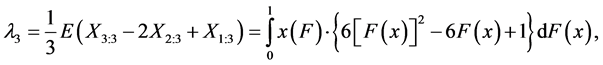
The letter “L” in “L-moments” indicates that the r-th L-moment λ_r is a linear function of the expected value of a certain linear combination of order statistics. The estimate of the r-th L-moment λ_r, based on the sample, is thus the linear combination of order data values, i.e. L-statistics. The first four L-moments of the probability distribution are now defined as

(6)

(7)

(8)

(9)

The probability distribution can be specified by its L-moments even if some of its conventional moments do not exist, the opposite, however, is not true. It can be proved that the first L-moment λ₁ is a location characteristic, the second L-moment λ₂ being a variability characteristic. It is often desirable to standardize higher L- moments λ_r, r ≥ 3, so that they can be independent of specific units of the random variable X. The ratio of L-moments of the r-th order of the random variable X is defined as

(10)

We can also define the function of L-moments which is analogous to the classical coefficient of variation, i.e. the so called L-coefficient of variation

(11)

The ratio of L-moments τ₃ is a skewness characteristic, the ratio of L-moments τ₄ being a kurtosis characteristic of the corresponding probability distribution. Main properties of the probability distribution are very well summarized by the following four characteristics: L-location λ₁, L-variability λ₂, L-skewness τ₃ and L-kurtosis τ₄. L-moments λ₁ and λ₂, the L-coefficient of variation τ and ratios of L-moments τ₃ and τ₄ are the most useful characteristics for the summarization of the probability distribution. Their main properties are existence (if the expected value of the distribution is finite, then all its L-moments exist) and uniqueness (if the expected value of the distribution is finite, then L-moments define the only distribution, i.e. no two distinct distributions have the same L-moments).

2.2. Sample L-Moments

L-moments are usually estimated by a random sample obtained from an unknown distribution. Since the r-th L-moment λ_r is the function of the expected values of order statistics of a random sample of the sample size r, it is natural to estimate it using the so-called U-statistic, i.e. the corresponding function of sample order statistics (averaged over all subsets of the sample size r, which may be formed from the obtained random sample of the sample size n).

Let be the sample and the ordered sample. Then the r-th sample L-mo- ment can be written as

(12)

Hence the first four sample L-moments have the form

(13)

(14)

(15)

(16)

U-statistics are widely used especially in nonparametric statistics. Their positive properties are the absence of bias, asymptotic normality and a slight resistance due to the influence of outliers, see [1] .

When calculating the r-th sample L-moment, it is not necessary to repeat the process over all sub-sets of the sample size r, since this statistic can be expressed directly as a linear combination of order statistics of a random sample of the sample size n.

If we assume an estimate of E(X_r:r) obtained with the use of U-statistics, it can be written as r·b_r−1, where

(17)

Namely

(18)

(19)

(20)

and so generally

(21)

Thus the first sample L-moments can be written as

(22)

(23)

(24)

(25)

We can therefore write generally

(26)

where

(27)

Sample L-moments are used in a similar way as sample conventional L-moments, summarizing the basic properties of the sample distribution, which are the location (level), variability, skewness and kurtosis. Thus, sample L-moments allow an estimation the corresponding properties of the probability distribution from which the sample originates and can be used in estimating the parameters of the relevant probability distribution. We often prefer L-moments to conventional moments within such applications, since sample L-moments―as the linear functions of sample values―are less sensitive to sample variability or measurement errors in extreme observations than conventional moments. L-moments therefore lead to more accurate and robust estimates of characteristics or parameters of the basic probability distribution.

Sample L-moments have been used previously in statistics, but not as part of a unified theory. The first sample L-moment l₁ is a sample L-location (sample average), the second sample L-moment l₂ being a sample L-variability. The natural estimation of L-moments (10) ratio is the sample ratio of L-moments

(28)

Hence t₃ is a sample L-skewness and t₄ is a sample L-kurtosis. Sample ratios of L-moments t₃ and t₄ may be used as the characteristics of skewness and kurtosis of a sample data set.

The Gini mean difference relates both to sample L-moments, having the form of

(29)

and the Gini coefficient which depends only on a single parameter σ in the case of the two-parametric lognormal distribution, depending, however, on the values of all three parameters in the case of the three-parametric lognormal distribution. For more details see, for example, [1] or [5] .

2.3. TL-Moments of Probability Distribution

An alternative robust version of L-moments is introduced in this subchapter. The modification is called “trimmed L-moments” and it is termed TL-moments. The expected values of order statistics of a random sample in the definition of L-moments of probability distributions are replaced with those of a larger random sample, its size growing correspondingly to the extent of the modification, as shown below.

Certain advantages of TL-moments outweigh those of conventional L-moments and central moments. TL-moment of the probability distribution may exist despite the non-existence of the corresponding L-moment or central moment of this probability distribution, as it is the case of the Cauchy distribution. Sample TL-mo- ments are more resistant to outliers in the data. The method of TL-moments is not intended to replace the existing robust methods but rather supplement them, particularly in situations when we have outliers in the data.

In this alternative robust modification of L-moments, the expected value E(X_r-j:r) is replaced with the expected value. Thus, for each r, we increase the sample size of a random sample from the original r to r + t₁ + t₂, working only with the expected values of these r modified order statistics by trimming the smallest t₁ and largest t₂ from the conceptual random sample. This modification is called the r-th trimmed L-moment (TL-moment) and marked as Thus, TL- moment of the r-th order of the random variable X is defined as

(30)

It is evident from the Expressions (30) and (1) that TL-moments are reduced to L-moments, where t₁ = t₂ = 0. Although we can also consider applications where the adjustment values are not equal, i.e. t₁ ≠ t₂, we will focus here only on the symmetric case t₁ = t₂ = t. Then the Expression (30) can be rewritten

(31)

Thus, for example, is the expected value of the median of the conceptual random sample of 1 + 2t size. It is necessary to note that is equal to zero for distributions that are symmetrical around zero.

For t = 1, the first four TL-moments have the form

(32)

(33)

(34)

(35)

The measurements of location, variability, skewness and kurtosis of the probability distribution analogous to conventional L-moments (6)-(9) are based on

The expected value E(X_r:n) can be written using the Formula (2). With the use of the Equation (2), we can express the right side of the Equation (31) again as

(36)

It is necessary to point out that represents a normal r-th L-moment with no respective adjustments.

Expressions (32)-(35) for the first four TL-moments (t = 1) may be written in an alternative way as

(37)

(38)

(39)

(40)

The distribution can be determined by its TL-moments, even though some of its L-moments or conventional moments do not exist. For example, (the expected value of the median of a conceptual random sample of sample size three) exists for the Cauchy distribution, despite the non-existence of the first L-moment λ₁.

TL-skewness and TL-kurtosis can be defined analogously as L-skewness and L-kurtosis

(41)

(42)

2.4. Sample TL-Moments

Let be a sample and an order sample. The expression

(43)

is considered to be an unbiased estimate of the expected value of the (j + 1)-th order statistic X_j+1:j+l+1 in the conceptual random sample of sample size (j + l + 1). Now we will assume that in the definition of TL-moment in (31), the expression E(X_r+t−j:r+2t) is replaced by its unbiased estimate

(44)

which is obtained by assigning j → r + t − j − 1 a l → t + j in (43). Now we get the r-th sample TL-moment

(45)

i.e.

(46)

which is an unbiased estimate of the r-th TL-moment Let us note that for each, the values x_i:n in (46) are not equal to zero only for r + t − j ≤ i ≤ n − t ?j, taking combination numbers into account. A simple adjustment of Equation (46) provides an alternative linear form

(47)

For r = 1, for example, we obtain for the first sample TL-moment

(48)

where the weights are given by

(49)

The above results can be used for the estimation of TL-skewness and TL-kurtosis by simple ratios

(50)

(51)

We can choose t = nα, representing the size of the adjustment from each end of the sample, where α is a certain ratio, where 0 ≤ α < 0.5. More about TL-moments, see [6] .

3. Results and Discussion

L-moments method used to be employed in hydrology, climatology and meteorology in the research of extreme precipitation, see, e.g. [5] , having mostly used smaller data sets. This study presents applications of L-moments and TL-moments to large sets of economic data, Table 1 showing the sample sizes of obtained household sample sets. Researched sampled sets of households constitute a reprezentative sample of the study population. The research variable is the net annual household income per capita (in CZK) in the Czech Republic (nominal income). The data collected by the Czech Statistical Office come from the EU-SILC survey (The European Union Statistics on Income and Living Conditions) spanning the period 2004-2007. In total, 96 income distributions were analyzed for all households in the Czech Republic as well as with the use of particular criteria: gender,

Table 1. Sample sizes of income distributions.

Source: Own research.

region (Bohemia and Moravia), social group, municipality size, age and the highest educational attainment. The households are divided into subsets according to their heads―mostly men. The head of household is always a man in two-parent families (a husband-and-wife or cohabitee type), regardless of the economic activity. In lone- parent families (a one-parent-with-children type) and non-family households whose members are related neither by marriage (partnership) nor parent-child relationship, a crucial criterion for determining the head of household is the economic activity, another aspect being the amount of money income of individual household members. The former criterion also applies in the case of more complex household types, for instance, in joint households of more two-parent families.

The value of α = 0.25 from the middle of the interval 0 ≤ α < 0.5 was used in this research. With only minor exceptions, the TL-moments method produced the most accurate results. L-moments was the second most effective method in more than half of the cases, the differences between this method and that of maximum likelihood not being significant enough as far as the number of cases, when the former gave better results than the latter. Table 2 represents distinctive outcomes for all 96 income distributions, showing the results for the total household sets in the Czech Republic. Apart from the estimated parameter values of the three-parametric lognormal distribution, which were obtained having simultaneously employed TL-moments, L-moments and maximum likelihood methods, Table 2 contains the values of the known test criterion χ², indicating that the L-moments method produced in two out of four cases―more accurate results than the maximum likelihood method, the most accurate outcomes in all four cases being produced by the TL-moments method.

For the years 2005, 2006 and 2007, an estimate of the value of the parameter θ (the beginning of the distribution, theoretical minimum) made by the maximum likelihood method is negative. This, however, may not interfere with good agreement between the model and the real distribution since the curve has initially a close contact with the horizontal axis.

Figure 1 and Figure 2 allow us to compare the methods in terms of model probability density functions in the given years (2004 and 2007) for the whole set of all households in the Czech Republic. It is clear from the three figures that the methods of TL-moments and L-moments produce very similar results, while the probability density function with the parameters estimated by the maximum likelihood method differs greatly from the model density functions constructed using TL-moments and L-moments methods respectively.

A comparison of the accuracy of the three methods of point parameter estimation is also provided by Figure 3. Data for the years 1992, 1996 and 2002 come from another statistical survey called Micronencsus, which was carried out in the Czech Republic until 2002. There are further 72 wage distributions. It shows the development of the sample median and theoretical medians of the lognormal distribution with the parameters estimated using the methods of TL-moments, L-moments and maximum likelihood for the whole set of households in the Czech Republic over the research period. It is also obvious from this figure that the curves indicating the development of theoretical medians of the lognormal distribution with the parameters estimated by TL-moments and L-moments methods fit more tightly to the curve representing the trajectory of the sample median compared to the curve showing the development of the theoretical median of the lognormal distribution with the parameters estimated by the maximum likelihood method.

4. Conclusions

A relatively new class of moment characteristics of probability distributions has been introduced in the present paper. They are the characteristics of the location (level), variability, skewness and kurtosis of probability distributions constructed with the use of L-moments and TL-moments that represent a robust extension of L-mo- ments. The very L-moments were implemented as a more robust alternative to classical moments of probability distributions. L-moments and their estimates, however, are lacking in some robust features that are associated with TL-moments.

Table 2. Parameter estimations of three-parametric lognormal curves obtained using three various methods of point para- meter estimation and the value of χ² criterion.

Source: Own research.

Figure 1. Model of probability densioty function of three-parametric lognormal curves in 2004 with parameters estimated using three various robust methods of point parameter estimation. Source: Own research.

Sample TL-moments are the linear combinations of sample order statistics assigning zero weight to a predetermined number of sample outliers. They are unbiased estimates of the corresponding TL-moments of probability distributions. Some theoretical and practical aspects of TL-moments are still the subject of both current and future research. The efficiency of TL-statistics depends on the choice of α, for example, have the smallest variance (the highest efficiency) among other estimates for random samples from the normal, logistic and double exponential distribution.

The above methods as well as other approaches, e.g. [7] or [8] , can be also adopted for modelling the wage distribution and other economic data analysis.

Figure 2. Model of probability densioty function of three-parametric lognormal curves in 2007 with parameters estimated using three various robust methods of point parameter estimation. Source: Own research.

Figure 3. Development of the model and sample median of net annual household income per capita (in CZK). Source: Own research.

Acknowledgements

This paper was subsidized by the funds of institutional support of a long-term conceptual advancement of science and research number IP400040 at the Faculty of Informatics and Statistics, University of Economics, Prague, Czech Republic.

Conflicts of Interest

The authors declare no conflicts of interest.

References

[1]	Hosking, J.R.M. (1990) L-Moments: Analysis and Estimation of Distributions Using Linear Combinations of Order Statistics. Journal of the Royal Statistical Society (Series B), 52, 105-124.
[2]	Serfling, R.J. (1980) Approximation Theorems of Mathematical Statistics. John Wiley & Sons, New York. http://dx.doi.org/10.1002/9780470316481
[3]	Adamowski, K. (2000) Regional Analysis of Annual Maximum and Partial Duration Flood Data by Nonparametric and L-Moment Methods. Journal of Hydrology, 229, 219-231. http://dx.doi.org/10.1016/S0022-1694(00)00156-6
[4]	Ulrych, T.J., Velis, D.R., Woodbury, A.D. and Sacchi, M.D. (2000) L-Moments and C-Moments. Stochastic Environmental Research and Risk Assessment, 14, 50-68. http://dx.doi.org/10.1007/s004770050004
[5]	Kysely, J. and Picek, J. (2007) Regional Growth Curves and Improved Design Value Estimates of Extreme Precipitation Events in the Czech Republic. Climate Research, 33, 243-255. http://dx.doi.org/10.3354/cr033243
[6]	Elamir, E.A.H. and Seheult, A.H. (2003) Trimmed L-Moments. Computational Statistics & Data Analysis, 43, 299-314. http://dx.doi.org/10.1016/S0167-9473(02)00250-5
[7]	Marek, L. (2011) Wage Development in the Czech Republic for the Past 16 Years. Proceedings of AIESA—Budovanie spolecnosti zalozenej na vedomostiach, Bratislava, 10-11 November 2011, 1-7.
[8]	Marek, L. and Vrabec, M. (2013) Model Wage Distribution—Mixture Density Functions. International Journal of Economics and Statistics, 1, 113-121.