Some Approximation in Cone Metric Space and Variational Iterative Method ()
1. Introduction
Fixed point theory has fascinated many researchers since 1922 with the celebrated Banach’s fixed point theorem. There exist a fast literature on the topic and this is a very active field of research at present (See [1-7]).
By using same definition and meaning in stating is also looking in [2] and [3] etc. we introducing the following results for needing. For convenience, the authors give the following definition and lemma (see the proof of theorem 3 [2])
Let  always be a real Banach space, and
  be the subset of
  is called a cone, if and only if:
(i)  is closed, nonempty, and
(ii) 
(iii) 
Given a cone we define a partial ordering
  with respect to
  by
by  if and only if
We shall write  to indicate
  but
but  while
while  implies
  int
int denotes the interior of
 .
.
Definition 1.1 Let  be a non-empty set in
 , and suppose the mapping
  satisfies:
(i)  for any
  and
and 
(ii)  for all
(iii)  for all
Then  is cone distance on
  is called a cone metric space.
It is obvious that cone metric space generalize the metric spaces.
Definition 1.2 Let  is said to be a complete cone metric space, if every Cauchy sequence is convergent in
Let  be a metric space. We denote by
  the family of non-empty closed bounded subset of
  Let
Let  be the Hausdorff metric on
 . That is for

where  is the distance from point
  to the sub-set
  An element
  is said to be a fixed point of a multi-valued mapping
Lemma 1.3 Suppose that  be a cone metric space and the mapping
  hold the sequence
  in
in  satisfying the following conditions:

and that is

Then the sequence  is a Cauchy sequence in
 .
.
2. Several Common Fixed Point Theorems
In recent years, the fixed point theory and application has rapidly development. Huang and Zhang [2] introduced the concept of a cone metric space that a element in Banach space equipped with a cone which induces a nature order partial order. In the same work, they investigated the convergence and that inequality and they extend the contractive principle to in partial order set s with some applications to matrix equations and common solution of integral equations.
Such theorems are very important tools for proving the existence and eventually the uniqueness of the solutions to various mathematical models (integral and partial differential equations, variations inequalities etc.).
First, we state following some extend conclusion ([3, 4]). Next, authors consider the variation iterative method to some integral and differential equations, and effective method ([5-8]) for examples and numerical test as some Fig case.
Now we first give common fixed point Theorem in similar method for two operators to extend Theorem 2.1 [2] with one operator case. Assume that  be a complete cone metric space.
Theorem 2.1 Let  be a complete cone metric space,
  a normal cone with normal constant
  Suppose that mappings
  satisfies the Contractive condition
 (2.1)
(2.1)
for each  where
where  is a constant
  Then
Then  has a unique common fixed point in
  And so for any
  the iterative sequence
  converges to the fixed point.
Corollary 2.2 Let  and
and  then we obtain that theorem 2.1 in [2].
In the same way, authors can extend theorem 4 [2], and omit again these stating.
3. Some Notes of Common Fixed Point
Theorem A (See Theorem 1 [3]) Assume that  be a complete cone metric space. Let mappings
  satisfying following Lipchitz conditions for any
 (3.0)
(3.0)
where  are nonnegative real value functions on
  such that

and that

Then there is a unique common fixed point in  for
for  and
and  and for any
  the iterative sequence
  convergent to the common fixed point of
Remark in [3], the example 2 illustrate this effect of meanings with this Theorem (non-expansion mapping, not contractive case that have uniqueness common fixed point). Look for multiple-value mappings in some case [5].
We can easy note Theorem A. Now we give complete this fixed point problem below.
Theorem 3.1 Same as the assume of theorem 1 [3]. Let  be a complete cone metric space, and there exists positive integer
  and mappings
  satisfying following Lipchitz conditions for any
  that is satisfy following inequality such that
 (3.1)
(3.1)
where  are non-negative real functions on
  If it holds,
Then there is a unique common fixed point in  for
for .
.
Proof By the proof of theorem 1 [3] that we known that  and
and  has a unique common fixed point
  and
and  from
from

then  is also common fixed point of
  and
and  Hence, we have
  by the uniqueness of them. In the same way, we know that
  that is,
  This
This  is a common fixed point of
 , and
, and

We have 
On the other hand, if  then clearly,
  in the same way, we know
  which a contradiction. So, we complete the proof of this theorem.
Theorem 3.2 Let  be a complete cone metric space, and mappings
  satisfying following Lipchitz conditions for any
  that is satisfy following inequality (
 nonnegative real constant)
 (3.2)
(3.2)
and

If  have not common fixed point each other, then the
  exist at least
  number fixed points in
Proof By the theorem 1 [3], we known that  and
and  has a unique common fixed point
  that is
  and that in the same way,

Then S have at least  number fixed points.
Corollary 3.3 Let  more positive integer cases in theorem 3.1.
Remark 3.4 (see corollary 5 [3]) Assume that  be complete cone metric space, and mappings
  satisfy following condition (
 non-negative real constant):
 (3.3)
(3.3)
And

then  must have uniqueness common fixed point, and for any
  iterative sequence
  convergent to the common fixed point

Here example 2 in [5] for non-expansion mappings, also have common fixed point case with important meanings.
4. Common Fixed Point of Four Mappings
Many authors have extended the contraction mapping principle in difference direction. Some extension of Banach’s fixed point theorem through the rational expression form with it’s inequality. The purpose of this section, is to establish some common fixed point theorem for four mappings in this space.
Theorem 4.1 Assume that  be a complete cone metric space, and mappings
  continuous and satisfying following conditions for any

and that inequality
 (4.1)
(4.1)
Then  have a unique common fixed point.
Proof Let  be an arbitrary point of
  and from
  we can choose a point
 such that
  Also
Also  we can choose a point
  such that
  In general, we can Choose
  and
and  define a sequence
  in
in  as follows,

Now, by (4.1) we have that

Similarly, we have

which implies that

Hence, it is well know that  is Cauchy sequence. From the
  is complete, then there exists
  such that the
  convergences to
  in
in  Since
Since  and
and  are subsequences of
  then it will convergence to same point u.
Next, from these  are continuous maps, we can obtain following results

It follows from  then we have
 and we get
  In the same reason,

we again obtain  By (4.1), if
  then
then

this is a contradiction. Hence, we have that

Let  then we obtain that

and

By (4.1), if  then
then

we get 
It is a contradiction. Thus, 
Similarly,

we get 
It is also a contradiction. Therefore, 
By (4.1), if  then
then

also a contradiction. Thus, we have

then this implies  for common fixed point of
 .
.
(Uniqueness) Let two points  be the difference common fixed point of
 .
.
By (4.1), we have

A contradiction in the above same reason, then this implies the uniqueness of common fixed point of .
.
Remarks
(i) As  we obtain special case.
(ii)  (Identity map),
  we get some special case.
Theorem 4.2 Assume that  be a complete cone metric space. Same as theorem 4.1, and satisfies these conditions below


for any
 (4.2)
(4.2)
Then  have a unique common fixed point.
Proof By theorem 4.1, we known that there is a unique fixed point  in
in  and
and 
Obviously,  This completes the proof of theorem 4.2.
5. Some Notes for Multi-Valued Mappings
According the direction of [5], we give out some coincidence point theorem of maps to extend theorem 2.1 and theorem 2.3 [5].
Let  be a strictly increasing function such that
(i) 
(ii)  for each
(iii)  for each
Now, we can easy obtain following theorems.
Theorem 5.1 Let  be a complete metric space and
  be multi-valued maps
 satisfying for each

where
 (5.1)
(5.1)
If  have not common fixed point each other, then there exist at least
  number fixed points in
Proof From theorem 2.1 [5], we known there exist  in
in  such that
  again for
  in
in 
The same way,

Since  not equality each other, then S have at least
  number fixed point. This completes the proof.
Theorem 5.2 Let  be a complete metric space and
  be multi-valued maps
 and
and  be a map satisfying
(i) 
(ii)  is complete(iii) there exists a function
  such that
 for every
  (5.2)
(5.2)
And for each 
 (5.3)
(5.3)
If  and
and  have not coincidence point each other, then the
  and
and  at least exist
  number coincidence points in
Proof From theorem 2.3 [5], we known there exist coincidence point  in
in  such that
  in the same way, the coincidence point
  in
in  with
with

Since

not equality each other, therefore  and
and  have at least
  number coincidence point. That is,

Then this completes the proof.
Corollary 5.3 Let  be a complete metric space and
  be multi-valued maps
 and
and  be a map satisfying
(i) 
(ii)  is complete(iii)
  for each
  where
where  such that
  for every
If  have not coincidence point each other, then
If we take  we easy get these conclusion below, where
  is the identity map on
Corollary 5.4 Let  be a complete metric space and
  be multi-valued maps
  and satisfying for each

where  such that
  for every
If  have not common fixed point each other, then the
  and
and  exist at least
 number points in
  That is case

Corollary 5.5 When , for each
  Then we get also similar conclusion case:
6. Solution of Integral Equation by VIM
Recently, the variation iteration method (VIM) has been favorably applied to some various kinds of nonlinear problems, for example, fractional differential equations, nonlinear differential equations, nonlinear thermo elasticity elasticity, nonlinear wave equations.
In this section, we apply the variation iteration method (simple writing VIM) to Integral-differential equations below (see [6,7]). To illustrate the basic idea of the method, we consider:

The basic character of the method is to construct functional for the system, which reads:

which can be identified optimally via variation theory,  is the nth approximate solution, and
  denotes a restricted variation, i.e.
  There is a iterative formula:

of this equation
 (*)
(*)
Theorem 6.1 (see theorem 3.1 [6]) Consider the iteration scheme  and
and
 . (6.1)
Now, for  to construct a sequence of Successive iterations that for the
  for solution of integral Equation
 .
.
In addition, we assume that

and  then if
  the above iteration converges in the norm of
  to the solution of integral equation
 .
.
Corollary 6.2 If  and
and

then assume  if
if  the above iteration converges in the norm of
  to the solution of integral equation
 .
.
Corollary 6.3 If  and
and

then assume  if
if  the above iteration converges in the norm of
  to the solution of integral Equation
 .
.
Example 6.4 Consider that integral equation
 (6.2)
(6.2)
where

then if  (See Figure 1(a)) then the iterative
  that convergent the solution of Equation (6.2) by corollary 6.2 of theorem 6.1. Therefore, we check that

From (6.1), we have that

Let

and

(See Figure 1(b), when n = 4).
The exact solution  Then we obtain exact solution below

Remark The exact solution  and approximate solution
  of Example 6.4 (See Figure 1(c)).
Example 6.5 We consider that integral equation
 (6.3)
(6.3)
From (6.1), we have that

We take

The exact solution  then we obtain exact solution below
By corollary 6.2 of Theorem 6.1, where that

Then the iterative sequence is convergent to the exact solution of the Equation (6.3).
In fact,

then if  the iterative sequence is convergent the solution of Equation (6.3).
Example 6.6 Consider that integral equation (
 positive integer),
 (6.4)
(6.4)
where  and we have that

We can take that
(k-positive integer), and

Inductively, we have

Then by Theorem 6.1 and simple computation, we obtain that

then if  the iterative is convergent the solution of integral equation (6.4) (Similar as examples case in [6, 7]).
7. Some Effective Modification and Numerical Test for [8]
In this section, we apply the effective modification method of He’s VIM to solve some integral-differential equations. In [6-8] by the variation iteration method (VIM ) simulate the system of this form

To illustrate its basic idea of the method, we consider the following general nonlinear system

the highest derivative and is assumed easily invertible,  is a linear differential operator of order less than,
  represents the nonlinear terms, and
  is the source term. Applying the inverse operator
  to both sides of above equation, we obtain

The variational iteration method (VIM) proposed by Ji-Huan He (see [6-8] recently has been intensively studied by scientists and engineers. the references cited therein) is one of the methods which have received much concern. It is based on the Lagrange multiplier and it merits of simplicity and easy execution. Unlike the traditional numerical methods. Along the direction and technique in [4,8] we may get more examples below.
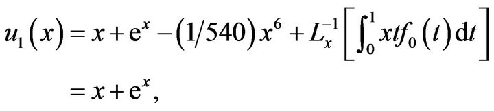
Example 7.1 (similar as example in [8]) Consider the following nonlinear Fredholm integral equation
 (7.1)
(7.1)
Applying the inverse operator  to both side of Equation (7.1), yields:

from 
So,

Inductively,

Then  is exact solution of (7.1). The numerical results are shown in Figure 2.
Example 7.2 Consider the following Volterra-Fredholm integral-differential equation
 (7.2)
(7.2)
Similar as example1 in this way, we easy get this solution.
According to the method, we divide into two parts defined
 and
and

By calculating this

So, we have

In fact, in this way

and

Writing

therefore, we have

Inductively,

And  Hence the
  is the exact solution of (7.2).
Example 7.3 Consider the following integral-differential equation
 (7.3)
(7.3)
where  In similar example1, we easy have it .
According to the method, we divide into two parts defined by

Figure 2. Figures of exact solution u(x) for Example 7.1.

Taking  then we have
where 
And the processes,

Thus,  then
then  is the exact solution of (7.3) by only one iteration leads to a solution. The numerical results are shown in Figure 3.
Example 7.4 (See example 2 in [8]) Consider the following partial differential equation
 (7.4)
(7.4)
Let that integer The modified methods:
Applying the inverse operator to both sides of (7.4) yields

where 
Here, we divide  into two parts defined by

Using the relation  we obtain

and so on

Hence,  is the exact solution of (7.4) and by only one iteration leads to that exact solution. Taking
  that is example 2 in [8].
The numerical results are shown in Figure 4.
Remark 7.5 Some solving integral-differential equations by VIM may see [9], and that some random Altman type inequality for fixed point results see [10].
The fixed point results of Multi-value mapping are also discussed in [11].
Remark 7.6 By [12], the authors consider the mixed problem for non-linear Burgers equation:
 (7.5)
(7.5)
The authors point out the problem describes physic phenomenon of motive quality and conservation of law in dynamic problem, it is important model in flow mechanics. Where  express the velocity of flow body,

Figure 3. Figures of exact solution u(x) for Example 7.3.
and  express the constant of motive flow body,
 -initial function.
Burger’s equation has attracted much attention. The approximation solution for this Burger’s equation is also interesting tasks.
8. Concluding Remarks
In this Letter, we give out new fixed point theorems in cone metric space and apply the variation iteration method to integral-differential equation, and extend some results in [3,6-8]. The obtained solution shows the method is also a very convenient and effective for some various non-linear integral and differential equations, only one iteration leads to exact solutions.
Recently, the impulsive differential delay equation and stochastic schrodinger equation is also a very interesting topic, and may look [11] etc.
9. Acknowledgements
This work is supported by the Natural Science Foundation (No.07ZC053) of Sichuan Education Bureau and the key program of Science and Technology Foundation (No.07zx2110) of Southwest University of Science and Technology.
The authors would like to thank the reviewers for the useful comments and some more better results.