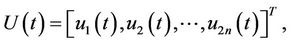
1. Introduction
In recent years, there has been an increasing interest in studying van der Pol coupled oscillator models. Synchronization, which is defined as an adjustment of rhythms due to a weak interaction, is one of the most interesting features displayed by coupled oscillators. It occurs in physics, chemistry, engineering, biology, social sciences, etc. [1-6]. For a delayed feedback model as follows:
 (1)
(1)
where ,
,  Jiang and Wei found that there were Bagdanov-Takens bifurcation, triple zero and Hopf-zero singularities for the equation under some restrictive conditions [7]. The following is a model of a self-excited system:
 (2)
(2)
Zhang and Gu [8] have shown that there exist the stability switches and a sequence of Hopf bifurcations occur at zero equilibrium when the delay varies. Recently, Zhang et al. [9] have considered a system of coupled electric circuit in a ring with n symmetrical van der Pol oscillators. By the Kirchhoff’s law, considering the time delay between the signal transmission of the oscillators, and after the normalization of the state variables and parameters, the model looks like this:
 (3)
(3)
where parameters c, p,  and
and  are positive constants. By choosing the delay as the bifurcating parameter, the authors have proposed some results of the Hopf bifurcations occurring at the zero equilibrium as the delay increases. Using the symmetric functional differential equation theories, the authors also have exhibited the multiple Hopf bifurcations, and their spatio-temporal patterns: mirror-reflecting waves, standing waves, and discrete waves.
However, if the time delay and the parameters c, p,  and
and  are different in each oscillator, in other words, if the system is not symmetric which may draw closer to reality, then we get the following system:
 (4)
(4)
We shall point out that with the method of bifurcation it will become very difficult to discuss the properties of the solutions of system (4) due to the complexity of parameters. In this paper, we use the analysis method to discuss the oscillatory behavior of the system (4). Simple criteria to guarantee the existence of oscillation of the system have been proposed.
2. Preliminaries
For convenience, set ,
,  , r = 1, 2, ∙∙∙, n. Then system (4) can be rewritten as follows:
 (5)
(5)
The nonlinear system (5) can be expressed in the following matrix form:
 (6)
(6)
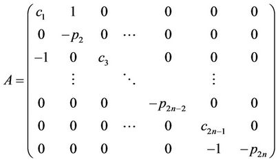
where
 .
.
Both A and B are 2n by 2n matrices, P(U) is a 2n by 1 vector.
 ,
,
 ,
,

Definition 1. A solution of system (4) is called oscillatory if the solution is neither eventually positive nor eventually negative. If  is an oscillatory solution of system (5), then each component of
  is oscillatory.
We adopt the following norms of vectors and matrices [10]:
 ,
,
 ,
,
 .
.
The measure  of the matrix A is defined by
 , which for the chosen norms reduces to

Note, that the linearization of system (5) about zero is the following:
 (7)
(7)
Or the matrix form
 (8)
(8)
Obviously, if the equilibrium point of system (7) (or (8)) is unstable, then this equilibrium point for system (5) (or (6)) is still unstable. Thus, in order to discuss the instability of the equilibrium point of system (5) (or (6)), we only need to focus on the instability of the equilibrium point of system (7) (or (8)). We first have Lemma 1. If for given parameter values of ,
,  , and
, and , the determinant of matrix (A + B) is not zero, then system (7) (or (8)) has a unique equilibrium point.
Proof. An equilibrium point  is a constant solution of the following algebraic equation
 (9)
(9)
Clearly,  is an equilibrium point. Since the determinant of matrix (A + B) is not zero, then Equation (9) has a unique equilibrium point, that is, the zero point.
3. Oscillation Analysis
Theorem 1. If linearized system (7) has a unique equilibrium point for given parameter values of ,
,  , and
, and  (i = 1, 2, ∙∙∙, 2n), assume that the following conditions hold for system (7) (or (8)):
(C1)
(C2) Both

and

hold, where
and
Then the unique equilibrium point of system (7) is unstable, implying that the unique equilibrium point of system (5) is also unstable. That is, system (5) generates permanent oscillations.
Proof. First consider the special case of system (7) as  (i = 1, 3, ∙∙∙, 2n − 1):
 (10)
(10)
If the unique equilibrium point is unstable for system (10), in other words, the trivial solution of (10) is unstable, then consider (10), for some , we have
 (11)
(11)
where  or
or ,
,  or −1 (i = 1, 2, ∙∙∙, 2n).
Hence for , we have
 (12)
(12)
where . Consider the scalar delay differential equation
 (13)
(13)
with . Based on the compareson theory of differential equation we get
  for
for . Thus, if the trivial solution
  is unstable, then the trivial solution
  is also unstable. It is not difficult to see that the trivial solution of (13) is unstable. Otherwise, the characteristic equation associated with (13) given by
 (14)
(14)
will have a real negative root, say , and
, and
 (15)
(15)
This means that
 (16)
(16)
where we use the inequality  for x > 0. The last inequality of (16) contradicts condition (C2). Thus the trivial solution of (13) is oscillatory. Now for time delays
  (i = 1, 3, ∙∙∙, 2n − 1), condition (C2) still holds. Therefore, the trivial solution of system (7) is oscillatory, implying the oscillations of the trivial solution about the equilibrium point of system (5).
Noting that  tends to zero as
  tends to infinity. Thus, Theorem 1 holds only for finite
 . In the following we provide a criterion for suitably large
  holds.
Theorem 2. If linearized system (7) has a unique equilibrium point for given parameter values of ,
,  , and
, and  (i = 1, 2, ∙∙∙, 2n), assume that there exists a suitably large positive number K such that the following conditions hold for system (7) (or (8)):
(C3) (17)
(17)
Then the unique equilibrium point of system (7) is unstable, implying that the unique equilibrium point of system (5) is also unstable. That is, system (5) generates permanent oscillations.
Proof. We will prove that the trivial solution of system (7) is unstable. It is sufficient to show that the characteristic equation associated with (13) given by (14) has a real positive root under the stated condition (C3). Since the Equation (14) is a transcendental equation, the characteristic values may be complex numbers. We claim that there exists a real positive root from condition (C3). Set
 (18)
(18)
then  is a continuous function of
 . Note that delay
 ,
,  ,
,  is bounded, then
 . On the other hand, from condition (C3) we have
 . Therefore, there exists
  such that
from the continuity of . In other words,
  is a real positive characteristic root of (14). The proof is completed.
Based on the property of characteristic roots of matrices A and B, we immediately have Theorem 3. If linearized system (8) as  (i = 1, 3, ∙∙∙, 2n − 1) has a unique equilibrium point for given parameter values of
 ,
,  , and
, and  (i = 1, 2, ∙∙∙, 2n), let
  and
and  be characteristic roots of matrices A and B, respectively. Suppose that the following conditions hold for the system (7) (or (8)):
(C4) There exists some real number pair ( ,
, ),
), satisfying
 . Then the trivial solution of (7) is unstable, implying that the unique equilibrium point of system (5) is also unstable. That is, system (5) generates permanent oscillations.
Proof. Consider the special case of system (7) as  (i = 1, 3, ∙∙∙, 2n − 1) and we get the following matrix form:
 (19)
(19)
Since  and
and  (i = 1, 2, ∙∙∙, 2n) are characteristic roots of matrices A and B, respectively, then the characteristic equation of (19) can be expressed as follows:
 (20)
(20)
Hence, we are led to an investigation of the nature of the roots for some j
 (21)
(21)
Since  and
and  is a real number, if
 , obviously, Equation (19) has a positive root
 , where
 . If
. If , noting that
  tends sufficiently small as
  tends suitably large and
 . We can also find a positive root
  for Equation (19), where
 . So the trivial solution of (19) is unstable, implying that the unique equilibrium point of system (5) is also unstable.
We point out that Theorem 3 for different  is still holds, and each criterion of the above theorem is a sufficient condition.
4. Simulation Result
We select parameter values c1 = 0.1, c3 = 0.2, c5 = 0.3; δ1 = 0.1, δ3 = 0.2, δ5 = 0.3; p2 = 2, p4 = 3, p6 = 4, and τ1 = 2.5, τ3 = 5, τ5 = 4.5, respectively. Consider the following three-node case:
 (22)
(22)
Thus, A and B are six by six matrices as follows:
 ,
,
 and
and
 (a)
(a) (b)
(b)
Figure 1. Oscillations of the solutions about the equilibrium point with time delays values: 2.5, 5, 4.5. (a) Oscillatory behavior of u1(t), u3(t), u5(t) about the equilibrium point, delays: 2.5, 5, 4.5; (b) Oscillatory behavior of u2(t), u4(t), u6(t) about the equilibrium point, delays: 2.5, 5, 4.5.
 (a)
(a) (b)
(b)
Figure 2. Convergence of the solutions about the equilibrium point with time delays values: 1.5, 1.7, 1.8. (a) Convergence of the u1(t), u3(t), u5(t) about the equilibrium point, delays: 1.5, 1.7, 1.8; (b) Convergence of the u2(t), u4(t), u6(t) about the equilibrium point, delays: 1.5, 1.7, 1.8.
In this case the characteristic roots of A are: α1 = 0.0533, α2 = −1.2702, α3 = −0.1510, α4 = −2.6490, α5 = −0.6298, α6 = −3.7533, and the characteristic roots of B are: β1 = −0.4268, β2 = −0.7732, β3 = 0, β4 = 0, β5 = 0, β6 = 0. There is a real number pair (α1 = 0.0533, β1 = −0.4268). From Theorem 3, system (22) is oscillatory (Figure 1). However, it is worth emphasizing that this oscillation is due to time delays. In other words, delay induced oscillation of system (22) under the above parameter values. Indeed, the trivial solution of this system is stable if without time delays. One can see that the characteristic values of matrix C = A + B when τi = 0 are: γ1 = −3.7047, γ2 = −2.5707, γ3 = −0.2060, γ4 = −0.8943, γ5 = −1.1122 + 0.3801i, γ6 = −1.1122 − 0.3801i. Also  is a higher order infinitesimal as
  tends to zero. So the unique equilibrium point of system
  is stable according to the property of the solution of ordinary differential equation. Also the time delay must approach a certain quantity, for the system to generate oscillations. Figure 2 indicates that the system is still stable when τ = 1.5.
5. Conclusion
In this paper, we use the analysis method to discuss the oscillatory behavior of a nonsymmetric system. Simple criteria to guarantee the existence of oscillation of the system were proposed. We have discussed the effect of time delays in the system. They can induce oscillation. Computer simulations indicate the theory’s accuracy.