Impact of Macroeconomic Volatility on Stock Market Volatility in Bangladesh

Md. Rafiqul Matin^*

School of Business & Economics, North South University, Dhaka, Bangladesh.

DOI: 10.4236/jfrm.2023.123013                

Abstract

This study investigates the impact of macroeconomic volatility on stock market volatility in Bangladesh employing GARCH and ARDL cointegration models using monthly data from January 1991 to December 2015. The findings confirm that none of the selected macroeconomic variables’ volatilities can significantly explain the long-and short-run stock market volatility. The variances of the residuals are found unstable for most of the period and the current volatility is more sensitive to its past values than to new surprises indicating market inefficiency. Although, the reform initiatives, undertaken following the catastrophe of 1996, have improved the volatility condition of the market, but the second catastrophe of 2010 has put a question mark on it. The outcomes of this study are expected to help regulators and policymakers in assessing the degree to which the stock market may need to be reformed.

Keywords

Stock Market Volatility, Macroeconomic Volatility, Conditional Variance, Volatility Clustering, GARCH Family Models, Autoregressive Distributed Lag (ARDL) Cointegration

1. Introduction

Most of the research has concentrated on the impact of macroeconomic variables on stock market return. Considering the number of crashes in stock markets and their impact on households, banks, and finally on the overall economy has increased the interest of regulators, practitioners, and researchers towards the impact of macroeconomic volatility on stock market volatility. The Dividend Discount Model (DDM), Capital Asset Pricing Model (CAPM), and Arbitrage Pricing Theory (APT) predict that any shock to economy is a source of systematic risk and there is no way that even a well-diversified portfolio like a market portfolio can shift it to anywhere else. Hence it is obvious that the shock to the macro economy must influence the stock market return (Chowdhury et al., 2006) .

Since macroeconomic variables are considered powerful factors to forecast the volatility of the stock market all over the globe, knowledge of the impact of macroeconomic volatility on stock market volatility is crucial to investors and policymakers. Moreover, the risk-return behavior analysis of the stock market is more important for developing countries, like Bangladesh, because these markets are very volatile. The higher volatility of these stock markets compels the investors to demand higher risk premium, which creates higher cost of capital and slows down the economic development (Mala & Reddy, 2007) .

In this backdrop, this study has examined the impact of macroeconomic volatility on stock market volatility in Bangladesh to investigate whether the stock market volatility can be explained by macroeconomic volatility or some other factors are creating the market volatility. There are five sections in this study. In Section 2, we have reviewed similar literature. The methodologies used in the study have been described in Section 3. The findings of the empirical investigations have been portrayed in Section 4. Finally, in Section 5, we have summarized the findings in the conclusion.

2. Literature Review

One of the earliest attempts to examine the impact of macroeconomic volatilities on stock market return volatility has been made by Schwert (1989) . His study found a positive linkage between macroeconomic volatility and stock market volatility, with the direction of causality being stronger from the stock market volatility to the macroeconomic volatility. He showed that the evidence of stock market uncertainty being higher during recessions than expansions when macroeconomic volatility could explain about half of the stock market volatility.

Liljeblom & Stenius (1997) examined the relationship between conditional stock market volatility and macroeconomic volatility using monthly data of Finland for the period from 1920 to 1991. Conditional monthly volatility was obtained from the Generalized Autoregressive Conditional Heteroskedasticity (GARCH) estimations. The results of the study indicated that the stock market conditional volatility was a predictor of macroeconomic volatility, as well as the converse. Tests of the joint and simultaneous explanatory power of the macroeconomic volatilities indicated that one-sixth to more than two-thirds of stock market conditional volatility was related to macroeconomic volatility.

Morelli (2002) examined the relationship between conditional stock market volatility and conditional macroeconomic volatility using UK data for the period from January 1967 to December 1995. Conditional volatilities were estimated using the well-known Autoregressive Conditional Heteroscedasticity (ARCH) and Generalized ARCH (GARCH) models. The macroeconomic variables used were industrial production, real retail sales, money supply, inflation, and exchange rate. The study confirmed that conditional macroeconomic volatilities did not explain the conditional stock market volatility.

Chowdhury et al. (2006) examined how the macroeconomic risk associated with industrial production, inflation, and exchange rate was reflected to the stock market return in the context of Bangladesh capital market. They used monthly data for the period from January 1990 to December 2004. They used GARCH model to find predicted volatility series for the variables considered in the study. Finally, Vector Autoregression (VAR) was employed to investigate the relation between the variables. The results showed significant unidirectional causality running from industrial production volatility to stock market volatility and from stock market volatility to inflation volatility, the latter being consistent with the theory. They concluded that there was relation between stock market volatility and macroeconomic volatility, but it was not as strong as suggested by standard finance theory. They recommended for further study.

Chinzara (2010) examined how the time-varying macroeconomic risk associated with industrial production, inflation and exchange rates were related to time-varying volatility in the South African Stock Market. The study focused on both aggregate stock market indices and sectorial indices to investigate whether the response to macroeconomic volatility varied across sectors. The study also distinguished between the different stages of the economy, i.e. times of tranquility and times of crisis. He used Augmented Autoregressive GARCH (AR-GARCH) and Vector Autoregression models. The findings showed that although the volatilities in inflation, gold price and oil price played a role, however, volatility in short-term interest rates and exchange rates were most important. The results also revealed that the financial crises had increased the volatility in the stock market.

Adeniji (2015) examined the relationship between stock market and macroeconomic volatility in a developing country, Nigeria. The study used cointegration, bivariate and multivariate VAR, Granger causality tests as well as regression analysis. The cointegration test confirmed a long-run relationship among the volatilities of the variables. The results of GARCH model showed that three out of the five macroeconomic variables chosen had significant impact on stock market volatility. The results also confirmed that stock market volatility was influenced by its own past volatilities as well as the new innovations. The results indicated that the volatility in GDP, inflation and money supply did not Granger-cause stock market volatility, but the volatility in interest rate and exchange rate Granger-caused stock market return volatility. The low explanatory power of the regression analysis was explained mentioning that this finding was admissible in the case of developing countries with the supremacy of non-institutional investors and the existence of information asymmetry problem among investors.

The risk return behavior analysis of stock market has become essential for Bangladesh considering two irrational fluctuations of Dhaka Stock Exchange (DSE) within one and a half decades, one in 1996 and other in 2010, which has created a severe impact on our socio-economic life. Furthermore, following the crash of 1996, several capital market development programs and automation initiatives of DSE have been undertaken to develop an efficient domestic capital market. In this perspective, it is also very important to examine whether these initiatives have improved the efficiency of the market. However, the comprehensive review of literatures has indicated that no such study has been made. Furthermore, a very few studies have used Autoregressive Distributed Lags (ARDL) approach, which is the most sophisticated cointegration technique, to examine the relationship between stock market volatility and macroeconomic volatility. This study has contributed a lot to fill up these gaps.

3. Methodology

The econometric models used for the estimation of conditional variances of the research variables and to examine the long- and short-term relationship between the conditional variances of stock market return and that of macroeconomic variables have been outlined in this section.

3.1. Sample Data

The stock market in Bangladesh and its economy has been going through numerous liberalization and deregulation processes since 1991. As a result, stock market capitalization, trading volume and the market index have shown phenomenal growth during this period. The market capitalization of Dhaka Stock Exchange (DSE) to GDP has increased from 0.94% in June 1991 to about 30.95% in June 2009 (Wahab & Faruq, 2012) . Also, the size of the economy has increased significantly. In this context, monthly data of DSE General Index, industrial production index, interest rate, inflation, exchange rate, money supply and gold price for the period from January 1991 to December 2015 i.e. 25 years data have been considered in this study. Data for longer period has been collected to capture long-term movements and to avoid the effects of settlement and clearing delays (Faff el al., 2005; Liow et al., 2006) . Later, data on stock market index are converted into continuously compounded returns by logarithmic transformation. The same logarithmic transformation is applied to the selected macroeconomic variables to capture the growth of the macroeconomic variables. The conditional volatilities of the variables are estimated using best fitted GARCH model. The research variables along with the descriptive statistics are presented in Appendix A.

3.2. Pre-Tests for Econometric Models

The first pre-condition for the volatility estimation is to check the stationarity of the first differences of the research variables. Given the relatively low power of unit root tests, multiple unit root tests have been applied to examine the stationarity and order of integration of each variables. For this purpose, the well-known Augmented Dickey Fuller (ADF), non-parametric Phillips-Perron (PP) tests and Kwiatkowski-Phillips-Schmidt-Shin (KPSS) test have been used. First, the ADF and KPSS tests are applied and if these two tests provide diverse results for any variable, then the PP unit root test has been used for final decision.

The second pre-condition for the volatility estimation is to examine the presence of autocorrelation and heteroscedasticity in the residuals of the ordinary least squares estimation. The Breusch-Godfrey Serial Correlation LM test and Autoregressive Conditional Heteroscedasticity (ARCH) test have been used for this purpose.

3.3. Autoregressive Conditional Heteroskedasticity (ARCH) Model

The Autoregressive Conditional Heteroskedasticity (ARCH) Model allows the conditional variance to vary with time and implies that present variance relies on the preceding squared error terms. The basic ARCH(q) model has two equations, the mean equation and the conditional variance equation. Both equations must be estimated simultaneously as the variance is a function of the mean. The presence of ARCH means the normal distribution is not always the best approximation. The mean and variance equations of an ARCH(q) process can be given as follows:

Mean equation: $Y_t={\pi }_0+{\displaystyle {\sum }_{i=1}^q{\pi }_i{Y}_{t-i}}+{\epsilon }_t$ where ${\epsilon }_t~iid\left(0,{\sigma }_t^2\right)$ (1)

Variance equation: ${\sigma }_t^2={\gamma }_0+{\displaystyle {\sum }_{j=1}^q{\gamma }_j{\epsilon }_{t-j}^2}$ (2)

In Equation (1) and Equation (2), Y_t−i is a set of regressors, and π_i and γ_j are coefficients and ε_t is independently distributed residual terms. One shortcoming of the ARCH model is that it resembles extra moving average pattern than autoregression. Later, Bollerslev (1986) has generalized the ARCH model which is known as GARCH model.

3.4. Generalized ARCH (GARCH) Model

The GARCH model is the workhorse of financial applications can be used to explain the volatility dynamics of almost every financial series (Engle, 2004) . The appeal of this model is its ability to capture both volatility clustering and unconditional return distribution with heavy tails. GARCH model considers conditional variance to depend on both autoregressive (AR) and moving average (MA) terms. The GARCH(p, q) in the simplest form can be written as:

Mean equation: $Y_t={\lambda }_0+{\displaystyle {\sum }_{i=1}^k{\lambda }_i{Y}_{t-i}}+{\epsilon }_t$ where ${\epsilon }_t~N\left(0,{\sigma }_t^2\right)$ (3)

Variance equation: ${\sigma }_t^2=\omega +{\displaystyle {\sum }_{i=1}^q{\alpha }_i{\epsilon }_{t-i}^2}+{\displaystyle {\sum }_{j=1}^p{\beta }_j{\sigma }_{t-j}^2}$ (4)

Equation (3) is an autoregressive process of order k, AR(k). Parameter λ₀ is the constant, k is the lag length, ε_t is the heteroskedastic error terms with its conditional variance given in Equation (4). In the conditional variance equation q is the number of ARCH terms, and p is the number of GARCH terms. However, the GARCH model has some weaknesses, the main one is that it does not capture asymmetry, which normally characterizes stock markets (Chinzara, 2010) . With this implication, the Exponential GARCH(EGARCH) proposed by Nelson (1991) is the first asymmetric GARCH model.

3.5. Exponential GARCH (EGARCH) Model

The mean equation of EGARCH model is same as the mean equation of GARCH model. However, the variance equation of EGARCH model is expressed in logarithmic term. This model is superior to GARCH model because it ignores the non-negativity constraint and it doesn’t impose any constraint on the parameters. The variance equation of EGARCH model can be written as:

Variance equation: $\ln {\sigma }_t^2=\omega +{\displaystyle {\sum }_{i=1}^q{\alpha }_i\left|\frac{{\epsilon }_{t-i}}{{\sigma }_{t-i}}\right|}+{\displaystyle {\sum }_{i=1}^q{\gamma }_j\frac{{\epsilon }_{t-i}}{{\sigma }_{t-i}}}+{\displaystyle {\sum }_{j=1}^p{\beta }_j\ln {\sigma }_{t-j}^2}$ (5)

In the variance equation α, γ and β are the parameters of the variance. On the left side of Equation (5) natural logarithm of series is taken to compose exponential leverage effect. The model is symmetric, if ${\gamma }_1={\gamma }_2=\cdots ={\gamma }_q=0$ , meaning that there is no leverage effect. However, γ_j < 0 indicates more impact of negative news on next period’s volatility than positive news, which indicates leverage effect, while γ_j > 0 represents the other way around. The second asymmetric GARCH model is the Threshold GARCH (TARCH) model proposed by Zakoian (1994) .

3.6. Threshold GARCH (TGARCH) Model

The threshold GARCH (TGARCH) studied by Glosten et al. (1993) , is simply a re-specification of the GARCH(1,1) model with an additional term in the conditional variance equation to account for asymmetry. The mean equation of TGARCH model is same as GARCH(1,1) model. However, the variance equation can be written as follows:

${\sigma }_t^2=\omega +{\alpha }_1{\epsilon }_{t-1}^2+\gamma D_{t-1}{\epsilon }_{t-1}^2+{\beta }_1{\sigma }_{t-1}^2$ (6)

where D_t−1 is the indicator function having the following values:

$D_{t-1}=\{\begin{array}{l}1,{\epsilon }_{t-1}<0\\ 0,{\epsilon }_{t-1}\ge 0\end{array}$

In Equation (6), γ is known as the asymmetry or leverage parameter. For good news ( ${\epsilon }_{t-1}>0$ ) and for bad news ( ${\epsilon }_{t-1}<0$ ). So, the good or bad news have differential effect on conditional variance. While good news has an impact of ${\alpha }_1$ , bad news has an impact of ${\alpha }_1+\gamma$ . Thus, if γ is significant and positive, then negative shocks have a larger effect on ${\sigma }_t^2$ than the positive shocks, while the other way around if γ is significant and negative.

The selection of the best fitted GARCH model for modeling volatility is an important issue. This study has used the Akaike Information Criterion (AIC) and Schwarz Information Criterion (SIC) as a goodness-of-fit tests to rank the different GARCH models to choose the best fitted GARCH model. Then the cointegration relationship between conditional volatility of the stock market return and that of the selected macroeconomic variables has been examined using Autoregressive Distributed Lags (ARDL) cointegration approach.

3.7. Autoregressive Distributed Lag (ARDL) Cointegration Approach

Pesaran et al. (2001) have developed a new approach to cointegration testing which is applicable irrespective of whether the regressors are I(0), I(1) or mutually cointegrated. The ARDL model considers a one-period lagged error correction term, which does not have restricted error corrections. Hence, the ARDL approach involves estimating the following Unrestricted Error Correction Model (UECM):

$\Delta Y_t=a_{0Y}+{\displaystyle {\sum }_{i=1}^k{b}_{iY}\Delta Y_{t-i}}+{\displaystyle {\sum }_{i=1}^k{c}_{iY}\Delta X_{t-i}}+{\theta }_{1Y}{Y}_{t-1}+{\theta }_{2Y}{X}_{t-i}+{\epsilon }_{1t}$

$\Delta X_t=a_{0X}+{\displaystyle {\sum }_{i=1}^k{b}_{iX}\Delta X_{t-i}}+{\displaystyle {\sum }_{i=1}^k{c}_{iX}\Delta Y_{t-i}}+{\omega }_{1X}{X}_{t-1}+{\omega }_{2X}{Y}_{t-i}+{\epsilon }_{2t}$

where Δ is the differenced operator, k represents the lag structure, Y_t and X_t are the underlying variables, and ε_1t and ε_2t are serially independent random errors with mean zero and finite covariance matrix. In the 1st UECM equation, where ΔY_t is the dependent variable, the null and the alternative hypotheses are:

$H_0:{\theta }_{1Y}={\theta }_{2Y}=0$ [there exists no long-run equilibrium relationship].

$H_0:{\theta }_{1Y}\ne 0,{\theta }_{2Y}\ne 0$ [there exists long-run equilibrium relationship].

Similarly, for the 2nd equation, where ΔX_t is the dependent variable, the null and alternate hypotheses are:

$H_0:{\omega }_{1X}={\omega }_{2X}=0$ [there exists no long-run equilibrium relationship].

$H_0:{\omega }_{1X}\ne 0,{\omega }_{2X}\ne 0$ [there exists long-run equilibrium relationship].

These hypotheses are tested using the F-test or t-test. These tests have non-standard distributions that depend on the sample size, the inclusion of intercept and trend variable in the equation, and the number of regressors. F-test has been used in this study. Pesaran et al. (2001) have discussed five cases with different restrictions on the trends and intercepts and the test statistics are compared to two asymptotic critical values rather than the conventional critical values. If the test statistic is above an upper critical value, the null hypothesis of ‘no long-run relationship’ can be rejected regardless of the orders of integration of the underlying variables. The opposite is the case if the test statistic falls below a lower critical value. If the sample test statistic falls between these two bounds, the result is inconclusive. ARDL crashes if any of the time series is integrated of order 2. So, it is important to know the order of integration of the variables under consideration. The Augmented Dickey-Fuller (ADF) and the Phillips and Perron (PP) unit root tests have been applied to check the stationarity and order of integration of the variables.

4. Findings of the Study

The results of ADF and KPSS tests (see Appendix B.1) reveal that all the series have unit root at level indicating that the series are nonstationary at level. The ADF test results show that except LM2 other series are stationary at first difference and LM2 is stationary at second difference. On the other hand, KPSS test results show that LCPI is stationary at first difference with trend and intercept but has unit roots with intercept, while LGDPRICE is stationary with intercept but has unit roots with trend and intercept. Nevertheless, both ADF and KPSS tests confirm that LCPI has significant trend and LGDPRICE has insignificant trend at first difference. These results reveal that both the series are stationary at first difference, meaning both ADF and KPSS tests confirm that except LM2 all variables are I(1). To resolve the diverse results related to LM2, PP unit root tests have been applied on LM2, the test results (see Appendix B.2) indicate that LM2 has unit root at level and stationary at first difference, meaning that the series is I(1). Thus, finally, we conclude that all the research variables are nonstationary at level and stationary at first difference, meaning that series are I(1).

Later, the residuals are tested for autocorrelation and heteroskedasticity using Breusch-Godfrey Serial Correlation LM Test and Autoregressive Conditional Heteroscedasticity (ARCH) Test respectively. The results of these tests indicate that the residuals are serially correlated and heteroskedastic. The plot of residuals (see Figure 1) also confirms volatility clustering of the residuals, meaning that the variance appears to be high during some periods and low in other periods. These results reveal that the nonlinear GARCH model to be applied for the estimation of the mean and variance equations. From the GARCH family model, the best fitted one has been chosen based on the lowest values of Akaike Information Criterion (AIC), Schwarz Information Criterion (SIC) and Log-likelihood test. The results (see Appendix C.1) have indicated that EGARCH(1,1,1) is the best model for our purpose. So, this model is used to estimate the mean and variance equations.

Figure 1. Residuals of ordinary least squares estimation.

The mean and variance equations are estimated with stock market return as dependent variable and growth of the macroeconomic variables as independent variables. The results of the model are shown in (see Appendix C.2). Several points can be noted from the results of EGARCH model. Firstly, the mean equation shows that growth of consumer price index (DLCPI), growth of money supply (DLM2) and growth of gold price (DLGDPRICE) are positively related to stock market return at 1 percent, 1 percent, and 10 percent significant level respectively. But the growth of exchange rate (DLEXR) is negatively related to stock market return at 5 percent significant level. On the other hand, growth of industrial production (DLIPI) and interest rate (DLINT) are not statistically significant in explaining stock market return. The results confirm that most of the macroeconomic variables can significantly explain stock market return.

Secondly, the conditional variance equation reveals the following facts:

• The ARCH term (α), and the GARCH term (β) are significant at 1 percent significant level, meaning that the conditional variance of the stock market return depends on both autoregressive (AR) and moving average (MA) terms;

• The estimated β is considerably higher than the α, which reveals that the stock market volatility is more sensitive to its lagged values than to new surprises;

• The sum of α and β is 0.9253 indicating that a shock persists for many future periods;

• The coefficient γ ≠ 0 and is significant at 1 percent level, which confirms the presence of asymmetric effect of good and bad news on the stock market volatility;

• The coefficient γ is positive, which discloses that the positive shock, created by good news, implies a higher next period conditional variance in the stock market return compared to the negative shock of same magnitude created by the bad news.

Finally, the ARCH-LM test results show that the null hypothesis of “no ARCH effect” can’t be rejected at 5 percent significant level indicating that the mean and variance equations are well specified.

4.1. Estimation of Conditional Variances of Research Variables

To estimate the conditional variance of each variable, two sets of univariate models are used. In the first model, three univariate GARCH models; namely GARCH(1,1), EGARCH(1,1,1) and TGARCH(1,1,1), are applied with constant only in the mean equation. In the second model, the mean equation includes a constant and a autoregressive term of order 1, AR(1), of the same variable. The best fitted model for estimation of the conditional volatility of each variable is chosen based on the Akaike Information Criterion (AIC) and the following conditions:

• If asymmetry coefficient (γ) is found significant, then the GARCH model is not considered because GARCH does not capture the asymmetry in the variable;

• If (α + β) > 1, then the series becomes explosive. An explosive series cannot be considered in the estimation process, so the model is excluded from the choice;

• The presence of heteroskedasticity in the residuals means the model is not well specified. So, if the residuals for a model shows heteroskedasticity, then that model is excluded from the choice. ARCH Lagrange Multiplier Test is used to examine the presence of heteroskedasticity in the residuals.

Based on the test results (see Appendix D), following models are selected for estimation of different variables, TGARCH for the stock market return; AR-GARCH for the growth of both industrial production index and inflation rate; AR-TGARCH for growth in both interest rate and money supply; AR-EGARCH for growth of exchange rate; EGARCH for growth of gold price. Then the EVIEWS software is used to estimate the conditional variances. Finally, the cointegration relationships between conditional volatility of the stock market return and that of the selected macroeconomic variables have been examined using Autoregressive Distributed Lags (ARDL) cointegration approach.

4.2. Cointegration Test Results

For cointegration test, the order of integration of the variables are checked using ADF and PP unit root tests. Before that, the stability of VAR of the variables are checked under two conditions; with trend and intercept, and with intercept only. If VAR is found stable, then the optimal lag length is determined. These lag lengths (see Appendix E.1) are used in the unit root tests. The results of the ADF and PP unit root tests (see Appendix E.2) reveal that none of the conditional variances is I(2).

The results reveal that the dependent variable has 1 lag, while among the independent variables, the growth of money supply has the highest 7 lags. So, 1 lag is set for dependent variable and 7 lags for regressors and has allowed the EVIEWS software to choose the optimal lag length for each of the variables within the set limits. Later, the log-likelihood ratio test for the joint hypothesis of unit root and deterministic linear trend is used to identify the trend specification of the variables. The results of the log-likelihood ratio test (see Appendix F) show that none of the variables has trend. So, in ARDL test, constant is included in the cointegration equation.

The results of ARDL specification along with the Pesaran Bounds Test (see Appendix G.1) indicate that the null hypothesis of “no long-run relationships exist” is rejected and the alternative hypothesis “there exists long-run relationship” is accepted at 1 percent significant level, which means there exists a long-run relationship between the conditional variances of stock market and six macroeconomic variables. The R2 value indicates that only 14.89 percent of the stock market volatility can be explained by the volatilities of the selected macroeconomic variables. The remaining 85.11 percent can be explained by the factors which have not been considered in the research. The F value is significant at 1% level, meaning that the regression coefficients are significant. The Durbin Watson statistic indicates that the residuals are uncorrelated.

As there exists a cointegration relationship, the cointegrating form and long-run relationship are examined. The results (see Appendix G.2) show that the conditional variances of growth of industrial production, consumer price index and exchange rate are positively related and that of interest rate, money supply and gold price are negatively related to the conditional volatility of the stock market return. But none of the coefficients is found statistically significant, which confirms that none of the selected macroeconomic volatilities can significantly explain the volatility of stock market in the long-run. Also, the short-run relationship show that all the independent variables have zero lag meaning that there is no short-run relationship between the variance of stock market and that of macroeconomic variables. However, the results of Error Correction Model (ECM) show that the error correction coefficient is significant and has the correct sign and approximately 29.11 percent of the short-run disequilibria is adjusted per month to bring about long-run equilibrium.

4.3. Viability and Stability Check of the Model

The results (see Appendix G) of Breusch-Godfrey Serial Correlation LM test, Breusch-Pagan-Godfrey test and Jarque-Bera statistic have indicated that the residuals are not serially correlated, heteroskedastic and not normally distributed meaning that the model is not a good fit model. Furthermore, the plot of CUSUM control chart (see Figure 2) has showed that the slope parameters are unstable around 1996 and the CUSUMSQ chart (see Figure 3) shows that the variances of the residuals are unstable for most of the period. So, the results indicate that the coefficients are not stable over most of the period, meaning that the relationship is not stable over the period.

The above results indicate that the cointegration model over the total sample period (from January 1991 to December 2015) is not a good fit model and the

Figure 2. Cumulative Sum (CUSUM) control chart.

Figure 3. Cumulative Sum of Squares (CUSUMSQ) control chart.

coefficients are not stable. In addition, relationships in the long- and short-run between stock market volatility and that of growth of macroeconomic volatilities is not statistically significant. These results may be due to the catastrophes of 1996 and 2010. However, findings also indicate that the catastrophe of 1996 is much more prominent than that of 2010, which has motivated us to check the volatility conditions of the stock market in between the catastrophes using data from January 2000 to December 2009. This period is named as the recovery period, because following the catastrophe of 1996, the Capital Market Development Program (CMDP) was undertaken to develop a fair, transparent, and efficient domestic capital market. Alongside, Dhaka Stock Exchange (DSE) started its journey of automation in 1998 and yet is striving for continuous upgradation of its trading platform to transform it into a modern world class exchange.

4.4. Volatility Modeling for the Recovery Period

To modeling volatility of the recovery period, the pre-test of the estimation process is carried out to check the stationarity of the variables. The first difference of the research variables in the recovery period are found stationary. Furthermore, the research variables are fitted into the Ordinary Least Squares (OLS) with the stock market return as dependent variable and the growth of macroeconomic variables as independent variables (see Appendix H). Then the residuals of the OLS are checked for autocorrelation and heteroskedasticity using Breusch-Godfrey Serial Correlation LM and Autoregressive Conditional Heteroscedasticity (ARCH) Tests respectively. The results of these tests show that the residuals are not serially correlated and not heteroskedastic at 5 percent significance level (see Appendix I). The results reveal that the GARCH model cannot be applied for estimation for this period because the GARCH can only be applied when the residuals are serially correlated and heteroskedastic. The plot of residuals (see Figure 4) also depicts that there is no volatility clustering during the period.

Figure 4. Residuals of ordinary least squares estimation for the recover period.

5. Conclusion

The mean equation of the EGARCH model has indicated that out of six macroeconomic indices only inflation, exchange rate and money supply can significantly explain the stock market return. Alongside, the variance equation has shown the presence of asymmetric effect of good and bad news on the stock market conditional volatility. The stock market return in Bangladesh does not have any leverage effect and the current market volatility is more sensitive to its past volatilities than to new surprises indicating the inefficiency of the market.

The residuals of Ordinary Least Squares (OLS) for the total sample period have shown serial correlation and heteroskedasticity, but for recovery period residuals are not serially correlated and homoscedastic. Also, the volatility clustering is observed in the total sample period, which is not found in the recovery period. This indicates that the reform initiatives taken after the catastrophe of 1996 has improved the volatility condition of the market. The results of cointegration test for the total sample period have confirmed that there exists a long-run cointegration relationship between the stock market volatility and the volatilities of the selected macroeconomic variables. However, none of the macroeconomic volatilities can significantly explain the stock market volatility. Also the cointegration results are not statistically viable and the coefficients are unstable over most of the period. Alongside, only a small percentage of stock market volatility can be explained by the selected macroeconomic variables’ volatilities indicating that the stock market volatility has been mostly driven by other factors, which have not been considered in this research.

These results are admissible for any market in developing countries like Bangladesh with the supremacy of non-institutional investors and the existence of information asymmetry problem among investors. These stock markets are partially driven by fad and fashions which are not related to the economic conditions. Alongside, the reforms measures, following the catastrophe of 1996, have improved the volatility condition of the stock market but the catastrophe of 2010 has put a question mark on it. So, the future research can investigate the volatility situation of the market considering the catastrophe of 2010. Finally, we expect that the outcomes of this study are expected to help regulators and policy makers in formulating different policies for ensuring and creating smooth trading and investment atmosphere, controlling market strategies and assessing the degree to which the stock market may need to be reformed.

Appendix A

A.1. Definition of Research Variables

A.2. Descriptive Statistics of the Research Variables

Appendix B

B.1. Results of ADF and KPSS Unit Root Tests

Notes: * denotes that coefficient is significant at 5% level.

B.2. Results of Phillips-Perron Unit Root Tests for Money Supply (LM2)

Notes: Critical values at 5% level for PP test with trend and intercept is −3.424977 and with intercept is −2.871029. * denotes that coefficient is significant at 5% level.

Appendix C

C.1. Test Statistics for Selection of Best Fitted GARCH Model

C.2. Results of EGARCH(1,1,1) Model

Notes: * and ** denote the significance of the coefficients at 5% and 10% level respectively.

Appendix D

Model Selection for Estimation of Conditional Variances

Notes: * and ** denote the significance of the coefficients at 1% and 5% level respectively.

Appendix E

E.1. Results of Optimal Lag and Unit Roots Test

E.2. Results of Unit Root Tests of Conditional Variances

Notes: Critical values at 5% level for ADF and PP tests with trend and intercept is −3.424977 and with intercept is −2.871029. * denotes that significance of coefficient at 5%.

Appendix F

Results of Log-Likelihood Ratio Test

Notes: This distribution follows Chi-squared distribution and the critical value for one degree of freedom is 3.841 at 5% level.

Appendix G

G.1. Results of Cointegration Test

G.2. Cointegrating Form and Long-Run Coefficients

Appendix H

Viability Check of the Model

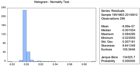
Normality Test of the Residuals

Appendix I

Ordinary Least Squares Estimation of the Recovery Period

Dependent Variable: DLDSEGEN

Method: Least Squares

Sample: 2000M1 2009M12

Included observations: 120

Notes: * denotes the significance of the coefficients at 1%.

NOTES

^*Adjunct Faculty (Professor).

Conflicts of Interest

The author declares no conflicts of interest regarding the publication of this paper.

References

[1]	Adeniji, S. O. (2015). An Empirical Investigation of the Relationship between Stock Market Prices Volatility and Macroeconomic Variables’ Volatility in Nigeria. European Journal of Academic Essays, 2, 1-12.
[2]	Bollerslev, T. (1986). Generalized Autoregressive Conditional Heteroskedasticity. Journal of Econometrics, 31, 307-327. https://doi.org/10.1016/0304-4076(86)90063-1
[3]	Chinzara, Z. (2010). Macroeconomic Uncertainty and Emerging Market Stock Market Volatility: A Case for South Africa. Rhodes University Working Paper No. 187, August 2010.
[4]	Chowdhury, S., Mollik, A., & Akhter, M. (2006). Does Predicted Macroeconomic Volatility Influence Stock Market Volatility? Evidence from the Bangladesh Capital Market. Department of Finance and Banking, University of Rajshahi, Working Paper.
[5]	Engle, R. (2004). Risk and Volatility: Econometric Model and Financial Practice. American Economic Review, 94, 405-420. https://doi.org/10.1257/0002828041464597
[6]	Faff, W. R., Hodgson, A., & Kremmer, L. M. (2005). An Investigation of the Impact of Interest Rates and Interest Rate Volatility on Australian Financial Sector Stock Return Distributions. Journal of Business Finance & Accounting, 32, 55-78. https://doi.org/10.1111/j.0306-686X.2005.00620.x
[7]	Glosten, L. R., Jagannathan, R., & Runkle, D. E. (1993). On the Relation between the Expected Value and the Volatility of the Nominal Excess Returns on Stocks. Journal of Finance, 48, 1779-1801. https://doi.org/10.1111/j.1540-6261.1993.tb05128.x
[8]	Liljeblom, E., & Stenius, M. (1997). Macroeconomics Volatility and Stock Market Volatility: Empirical Evidence on Finnish Data. Applied Financial Economics, 7, 419-426. https://doi.org/10.1080/096031097333538
[9]	Liow, H. K., Ibrahim, F. M., & Huang, Q. (2006). Macroeconomic Risk Influences on the Property Stock Market. Journal of Property Investment and Finance, 24, 295-323. https://doi.org/10.1108/14635780610674507
[10]	Mala, R., & Reddy, M. (2007). Measuring Stock Market Volatility in an Emerging Economy. International Research Journal of Finance and Economics, 8, 126-133.
[11]	Morelli, D. (2002). The Relationship between Conditional Stock Market Volatility and Conditional Macroeconomics Volatility Empirical Evidence Based on UK Data. International Review of Financial Analysis, 11, 101-110. https://doi.org/10.1016/S1057-5219(01)00066-7
[12]	Nelson, D. B. (1991). Conditional Heteroskedasticity in Asset Returns: A New Approach. Econometrica, 59, 347-370. https://doi.org/10.2307/2938260
[13]	Pesaran, M. H., Shin, Y., & Smith, R. J. (2001). Bounds Testing Approaches to the Analysis of Level Relationship. Journal of Applied Economics, 16, 289-326. https://doi.org/10.1002/jae.616
[14]	Schwert, G. W. (1989). Why Does Stock Market Volatility Change over Time? The Journal of Finance, 44, 1115-1153. https://doi.org/10.1111/j.1540-6261.1989.tb02647.x
[15]	Wahab, M. A., & Faruq M. O. (2012). A Comprehensive Study on Capital Market Developments in Bangladesh. Research Department, Bangladesh Bank.
[16]	Zakoian, J. M. (1994) Threshold Heteroskedastic Models. Journal of Economic Dynamics and Control, 18, 931-955. https://doi.org/10.1016/0165-1889(94)90039-6