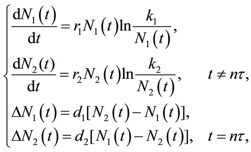
A Single Species Model with Symmetric Bidirectional Impulsive Diffusion and Dispersal Delay ()
1. Introduction
Species dispersal in patchy environment is one of the most prevalent phenomena of nature, and many empirical works and monographs on population dynamics in a spatial heterogeneous environment have been done. The persistence and extinction for ordinary differential equation and delayed differential equation models were investigated in [1-6]. Global stability of equilibrium and periodic solution for diffusing model were studied in [7-12]. Particularly, the predator-prey system with the prey dispersal also were studied in [13-15]. Regretfully, in all of above population dispersing systems, they always assumed that the dispersal occurs at every time. For example, in [16], Mahbuba and Chen proposed the following two patches single species diffusion system:
 (1.1)
(1.1)
where  presents the dispersal rate from patch j to patch i at time t. The form of the dispersal established in this model is continuous, that is, the dispersal is always happening at any time.
Actually, real dispersal behavior is very complicated and is always influenced by environmental change and human activities. It usually occurs stochastically or discontinuously [17], and it is often the case that species dispersal occurs at some transitory time slots when individuals move among patches to search for mates, food, refuge, etc.
Animal movements between regions or patches of habitat are rarely continuous in time. They may occur during short time slots within seasons or within the lifetimes of animals. This short-time scale dispersal is more appropriately assumed to be in the form of impulses in the modeling process, in order to be in much better agreement with the real ecological situation. For example, when winter comes, birds will migrate between patches in search for a better environment, whereas they do not diffuse in other season, and the excursion of foliage seeds occurs during a fixed period of time every year. Thus impulsive dispersal provides a more natural description. With the developments and applications of impulsive differential equations, theories of impulsive differential equations have been introduced into population dynamics, and many important studies have been performed [18-24].
In [19], Wang and Chen studied the following autonomous single-species model with impulsively bidirectional diffusion:
 (1.2)
(1.2)
where 
 presents the population density or size at time t,
  is the intrinsic growth rate of the population
 , and
, and  is the dispersal rate in the ith patch.
 , where
  represents the density of population in the ith patch immediately after the nth diffusion pulse at time
 , while
  represents the density of population in the ith patch before the nth diffusion pulse at time
  (
( the period of dispersal between any two pulse events is a positive constant,
 ). It is assumed here that the net exchange from the jth patch to ith patch is proportional to the difference
  of population densities. The dispersal behavior of populations between two patches occurs only at the impulsive instants
 . Obviously, in this model, species N inhabits respectively two patches before the pulse appears, when the time at the pulse comes, species N both in two patches disperse from one patch to the other. Sufficient criteria were obtained for the permanence, existence, uniqueness and global stability of positive periodic solutions by using discrete dynamical system theory.
It is well known that the time delay is quite common for a natural population. In order to reflect the dynamical behaviors of models that depend on the past history of system, it is often necessary to take the effect of time delay into account in forming a biologically meaningful mathematica model. Delay differential equations have attracted a significant interest in recent years due to their frequent appearance in a wide range of applications. They serve as mathematical models describing various phenomena in physics, biology, physiology, and engineering, see, e.g., [25,26] and references therein. There has been an extensive theoretical works on delay differential equations in the past three decades. The research topics include global asymptotic stability of equilibria, existence of periodic solutions, complicated behavior and chaos, see, e.g., [8,14,27,28].
Zhang and Teng in [14] introduced the following two species time-delayed predator-prey Lotka-Volterra type dispersal system with periodic coefficients (1.3):
where ,
,  denote the population density of prey species in ith patch and y is the population density of predator species. In this paper, the authors took dispersal delay into account, however, they assumed that the dispersal is continuous. Sufficient conditions on the boundedness, permanence and existence of positive periodic solution for system (1.3) are established.
 (1.3)
(1.3)
Recently, the application of impulsive delay differential equations to population dynamics is also an interesting topic since it is reasonable and correct in modelling the evolution of population, such as pest management [29].
However, in all of the impulsive dispersal models studied up to now, there are few papers considering the dispersal delay, which is really a pity. Actually, in the real world, the migration between patches is usually not immediate, that is, dispersal processes often involve with time delay. For example, elks move from higher to lower elevations to escape cold in winter, and ungulates migrate annually among grazing areas to following spatio-temporal changes in rainfall. In these cases, movement is unidirectional during each migration period and takes place over fairly short time periods. Obviously, this kind of dispersal delay between patches extensively exists in the real world. Therefore, it is a very basilic problem to research this kind of population dynamic systems.
Motivated by the calculation hereinbefore, in this paper, we consider the following impulsive dispersal system with dispersal delay:
 (1.4)
(1.4)
where we suppose that the system is composed of two patches connected by diffusion. The pulse diffusion occurs every  period, the system evolves from its initial state without being further affected by diffusion until the next pulse appears;
  stands for the time delay, that is, a period of species N disperse between patch i and j.
 ,
,  and
and  are positive constants.
The organization of this paper is as follows. In section 2, as preliminaries, the definition of permanence and some useful lemmas are introduced. From discrete dynamic system theory, we establish the stroboscopic map of system (1.4), by which we can obtain the dynamical
behaviors of it. The theorem on the permanence for system (1.4) is stated and proved in Section 3. In section 4, the existence and uniqueness of positive periodic solution for the system are obtained by the intermediate value theorem. In Section 5, the global stability of the positive periodic solution for system is established by the discrete dynamic system theory in [30]. Finally, we give a brief discussion and our theoretical results are conformed by numerical simulations.
2. Preliminaries
For any fixed , let
, let  be a piecewise continuous function such that
  is continuous in
 ,
, 
and  exist. For any fixed
 let
let  denote the Banach space of all such piecewise continuous functions
  with the norm
 . Further, let
 for all
 and
and  for
for .
.
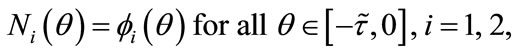
Motivated by the biological background of system (1.4), in this paper we always assume that all solutions of system (1.4) satisfy the following initial conditions:
 (2.1)
(2.1)
where . For any
 , by the fundamental theory of impulsive functional differential equations [31,32], system (1.4) has a unique solution
  satisfying the initial conditions (2.1). It is easy to prove that the solution
  of system (1.4) is positive, that is,
 in its maximal interval of the existence.
Definition 2.1. System (1.4) is said to be permanent, if there are positive constants  and
and  such that

for any positive solution  of system (1.4).
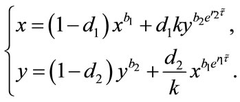
Next, to study the permanence, existence and uniqueness of positively periodic solutions for system (1.4), we take , which on substituting into (1.4) becomes:
 (2.2)
(2.2)
By integrating and solving the first two equations of system (2.2) between pulse, we have
 (2.3)
(2.3)
Similarly, considering the last two equations of system (2.2), we obtain the following stroboscopic map of system (2.2):
 (2.4)
(2.4)
where

Remark 2.1. System (2.4) is a difference system. It describes the densities of population in two patches at a pulse in terms of values at the previous pulse. We are, in other words, stroboscopically sampling at its pulsing period. The dynamical behavior of system (2.4), coupled with (2.3), determine the dynamical behavior of system (1.4). In the following sections, we will focus our attention on system (2.4), and investigate various aspects of its dynamical behavior.
Next, In order to establish the permanence of system (2.4), we introduce the following two lemmas.
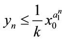
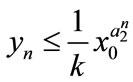
Lemma 2.1 Without loss of generality we assume that . Let
. Let ,
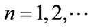
, . For
. For , if
, if , then we have:
Case (1). If ,
,  , then
 ,
,  ,
, ; if
; if ,
,  , then
 ,
,  ,
, .
.
Case (2). If ,
,  , then
 ,
,  ,
, ; if
; if ,
,  , then
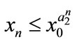 ,
,  ,
, .
.
Proof. We first prove that the first part of Case (1) holds. If ,
,  , then from (2.4), we have
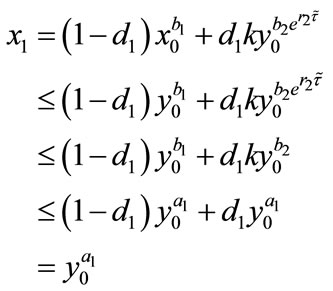
and

Hence, the first part of Case (1) is true for . Next, we assume that the conclusion holds for
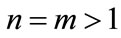 , that is,
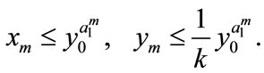
Then, for , we get


From the above discussion, we can see that the first part of Case (1) is true. Similarly, we can prove that the second part of Case (1) and the Case (2) are also true, so we omit the proof. This completes the proof.
By the same method, we have the following Lemma 2.2.
Lemma 2.2 Without loss of generality we assume that . Let
. Let ,
, . For
. For ,
,  , if
, if , then we have:
Case (1’). If ,
,  , then
 ,
,  ,
, ; if
; if ,
,  , then
 ,
,  ,
, .
.
Case (2’). If ,
,  , then
 ,
,  ,
, ; if
; if ,
,  , then
 ,
,  ,
, .
.
Lastly, in order to establish the global stability of positively periodic solution, we introduce the following lemma:
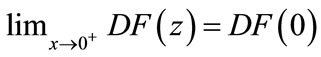
Lemma 2.3 ([30]) Let  be continuous,
  in int
 , and suppose
  exists with
 . In addition, assume
(a) 
(b) 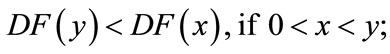
If , let
, let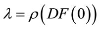 . If
. If , then for every
 ,
,  as
as ; if
; if , then either
  as
as  for every
 ; or there exists a unique nonzero fixed point q of F. In the latter case,
  and for every
 ,
, 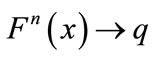 as
as .
.
If , then either
 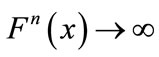 as
as  for every
  or there exists a unique fixed point q of F. In the latter case,
  and for every
 ,
,  as
as .
.
3. Permanence
The permanence plays an important role in mathematical ecology since the criterion of permanence for ecological systems is a condition ensuring the long-term survival of all species. In this section, we prove system (2.4) is permanent which will imply the permanence of system (1.4).
Theorem 3.1 For ,
,  , system (2.4) is permanence if
 .
.
Proof. Since ,
,  ,
,  ,
,  , we obtain

By Lemmas 2.1 and Lemmas 2.2, we can get that for , large enough, there exists constants
 ,
,  such that
  and
and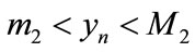 , that is,
  and
and  This means system (2.4) is permanent. The proof of Theorem 3.1 is completed.
4. Existence and Uniqueness of Positive Periodic Solution
In this part, we will prove the existence and uniqueness of the fixed points of system (2.4), which means that system (1.4) has a uniquely positive periodic solution.
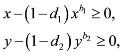
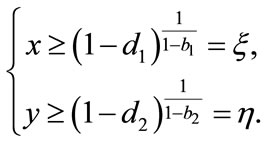
Theorem 4.1 There exists a unique positive fixed point  of system (2.4) provided that


Proof. Corresponding to (2.4), let us consider the following system (4.1):
 (4.1)
(4.1)
From (4.1), we have
 (4.2)
(4.2)
hence
 (4.3)
(4.3)
From (4.1), we obtain
 (4.4)
(4.4)
Since
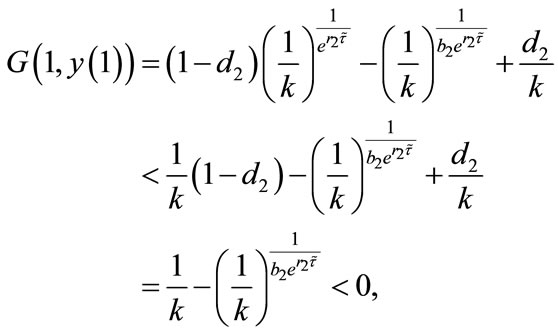

by the intermediate value theorem, we can see that there exists  such that
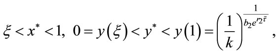

It follows from (4.3) that we obtain
 (4.5)
(4.5)


By (4.2) and assumption, we have ,
, 
 ,
,
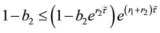 . So, we obtain
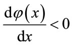 , which implies that
  is a decreasing function on the interval
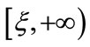 .
.
Since
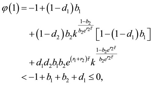


using the intermediate value theorem, there exists a unique point  such that
 . Besides,

thus

which, together with , leads to
 ,
,  By
By ,
,  we have that there exists a unique point
  such that
 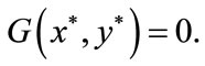 The proof is completed.
5. Global Stability
Now, we will prove that the positive fixed point  of system (4.1) is globally stable by using Lemma 2.3, which means that the positive periodic solution of system (1.4) is globally stable.
Theorem 5.1 For every ,
,  as
as .
.
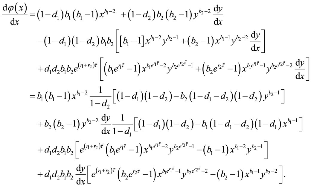
Proof. For any small ,
,  , we make the change of variable

and get the map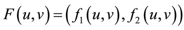 , that is,
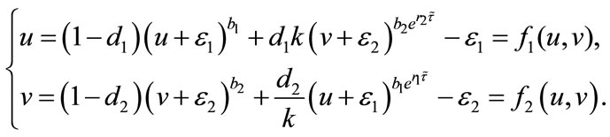 (5.1)
(5.1)
Now, we show that  satisfies the hypotheses of Lemma 2.3. It is easy to see that
 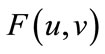 is continuous
  in
in , and
, and .
.
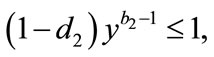
Since


so . If
. If , then
 ; if
; if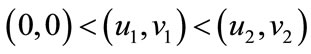 , then
  . Obviously, Theorem 5.1 satisfies all the conditions of Lemma 2.3, then for every
 , we have
 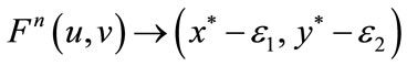 as
as . Corresponding to
  coordinate, this means for
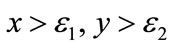 , the system (4.1) trends to unique fixed point.
Besides, we have 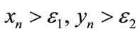 for initial value
  as
as .
.
From the above analysis, we can know that for every , the trajectory of system (2.4) will trend to
 . This completes the proof.
6. Numerical Simulation and Discussion
In this paper, we have investigated a single species model with symmetric bidirectional impulsive diffusion and dispersal delay, the criteria for the permanence, existence, uniqueness and stability of positive periodic solution are established.
Firstly, in Table 1 we show the effect of time delay on the populations. By simple calculating, we can get
provided . And
. And

So, all conditions of Theorem 3.1 and Theorem 4.1 hold, which means system (2.2) is permanent and has an unique globally stable periodic solution. From Figure 1, we can see that in this four different cases the species x
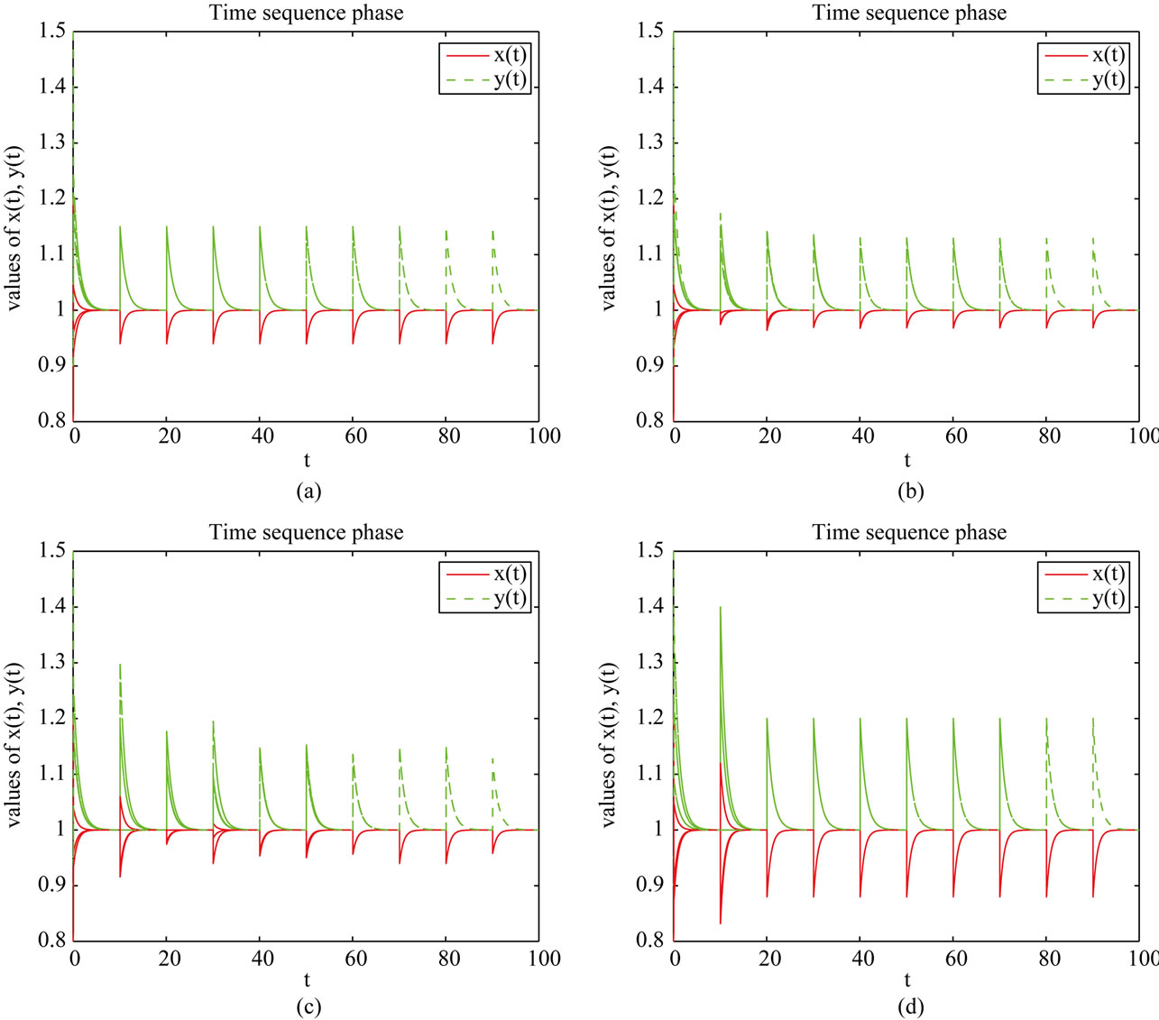
Figure 1. Dynamical behavior of system (2.2). Here, we take three sets of initial values (0.8, 1.5), (1.2, 0.9), (1.05, 0.95).

Table 1. Parameter values used in the simulations of model (2.2).
and y are both permanent. Moreover, the longer the duration of the time delay ( ), the larger the limit inferior of x and the lower the limit superior of y (see Figures 1(a) and (b)). This implies the case with dispersal delay is beneficial to species x living and harmful to species y.
Next, in Table 2, if , species x and y are both permanent, too (see Figure 1(c)). If we take
 ,
,  ,
,  , and keep other parameters unchanged in Table 1, then
 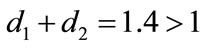 which purports that it does not satisfy the condition of Theorem 3.1, but we also get species x and y are both permanent (see Figure 1(d)). Therefore,
  and
and  are sufficient conditions for the permanence of system (1.4), but not a necessary ones.
Furthermore, in Table 3, by numerical simulations (see Figures 2(a) and (b)), we find that all of the solutions of system (2.2) which through these initial points will converge to the positive periodic solution. Therefore, we can conclude that under the assumptions of Theorem (4.1) system (2.2) has a unique positive periodic solution which is globally asymptotically stable. In addition, the periodic solution is lager in Case II than in Case I which indicates that the duration of the time delay is beneficial to species x living again. Comparing Figures 2(c) and (d), we realize that system (1.4) with time delay is more complicated than without.

Figure 2. Dynamical behavior of system (2.2). we take a series initial points, such as (0.9, 0.88), (0.92, 0.9), (1, 1.03).

Table 2. Simulations of model (2.2).

Table 3. Simulations of model (2.2).
7. Acknowledgements
This work was supported by the National Natural Science Foundation of P.R. China (10901130, 10961022), Natural Science Foundation of Xinjiang Province of China (2012211B07), the China Scholarship Council.
NOTES