On the Artificial Equilibrium Points in the Circular Restricted Problem of 2 + 2 Bodies

Kumari Ranjana¹, Vijay Kumar²

¹Lakshmibai College, University of Delhi, New Delhi, India.
²L S College, B R A Bihar University, Muzaffarpur, India.

DOI: 10.4236/ijaa.2017.74020                

Abstract

The present work studies the stability condition of central control artificial equilibrium points of the planar circular restricted problem of 2 + 2 bodies (PCRP2 + 2B) and also its variant when the shape of larger mass is taken to be an oblate spheroid. We find that the paper will be of great application in choosing an artificial equilibrium point (AEP) in the neighbourhood of numerous planets e.g. Jupiter or the bodies which provide a model of the problem studied. The minimum thrust will save a quantum of energy to be applied to have an arbitrary point as a chosen starter. For solar sailing and magnetic force this minimum thrust will be of great use.

Keywords

(PCRP2 + 2B), AEP, Stability, Minimum Thrust

1. Introduction

The 2 + 2 body problem has been introduced by [1] as a model for the dynamical behavior of two interacting bodies of comparable mass under the gravitational influence of two much more massive primaries unperturbed by the small bodies. Due to various expected celestial reasons the analytical means of assessing the stability of binary asteroid orbits became a celestial problem which engaged many authors e.g. [1] [2] [3] [4] and many others. Up to our recent knowledge it has been shown by [4] that the stability is not possible even for a finite time and so it is not guaranteed for long, with the conclusion [3] [4] it was felt that there was no stable region in the neighborhood of an equilibrium solution of 2 + 2 bodies for a long time. However later in the paper [5] it was shown that there does exists stability region in the neighbourhood of a triangular libration point and the conclusion showed that space stations can be launched in the neighbourhood of this stable libration point and hence to seek an artificial equilibrium point with the aid of solar sail or the magnetic device is possible. With this possibility we have investigated the minimum thrust to have the (AEP) for the (CRP2 + 2B) when all the four bodies are point masses and in its variant form when one of the larger mass is of the shape of an oblate spheroid.

The problem under our investigation is really a generalization of the classical restricted problem of three bodies (CRP3B). In nature we find a system of primary masses interacting with each other and their motion is completely determined by their interactions. On the other hand they are not influenced by the presence of the minor bodies. For example, we may consider the motion of asteroids or comets in the gravitational field of the Jupiter and Sun or that lunar probe in the gravitational field of Earth and Moon. In these problems we find that the presence of the minor bodies does not affect the motion of primaries while the primaries affect the latter ones. The (RP2 + 2B) has been investigated by many others as referred above.

Here we shall investigate the presence of AEP with the application of propellant force exerted by solar sail or other mechanical devices for the (CRP2 + 2B). The use of solar sails is not a new idea, but it is being exercised since the last many years. The names of [6] [7] are worth to be named to be the founders of idea. Later on, many investigators made use of different kinds of solar sails. [8] devised different types of solar sails and he is still engaged in having a more manageable and complicated one and less costly. Really solar sail is a proposed form of space craft propulsion that takes advantages of the radiation pressure to propel a space craft by means of a larger membrane mirror. The impact of the photons emitted by the sun on the surface of the sail and its further reflection accelerates the space craft. Although the acceleration produced by the solar radiation pressure is smaller than the one achieved by the traditional propulsion system, but this one is continuous and non-exhausting. So this makes long-time missions more accessible [7] . In addition many hybrid sails have also been devised recently to explore and with different aims to achieve.

In the present paper we have studied the existence of (AEP) for the (RP2 + 2B). We foresee a great prospect of achievement with the present study. The stationing of the space-crafts in the stable region of the libration point with the minimum thrust is our main aim behind the present study. It is proposed that two space-crafts may be stationed in the neighborhood of stable libration points with Earth &Moon or with Jupiter and Sun or similarly other planetary bodies for the primaries. The result can be utilized to study the motion of minor planets or comets.

Here we have chosen the model of (PRP2 + 2B) as introduced by [1] . As stated above in the first paragraph, the stability problem of the referred problem had also been studied [4] as well, but it was proved that there is no stable region and hence the question of stationing of space-craft did not arise. The stability region has been shown only by [5] by numerical calculation in the neighborhood of particular triangular libration point which made possible of imaging artificial equilibrium point having stability.

In the present work we consider the motion of two minor bodies with negligible mass interacting with each other but not affecting the two primaries interacting with each other and also affecting the motion of minor bodies. While studying the motion when one of the larger mass is of the shape of an oblate spheroid, we have used the result [2] [3] letting that the orbital planes of the centre of the different bodies coincide with their equatorial planes. With this assumption the common equatorial plane has been chosen for the xy-plane when the motion is assumed to take place. In course of studying the stable region it has been seen [9] that the motion of the minor mass m₁ may be taken independent of the motion of m₂ and similarly the motion of m₂ may be taken independent of m₁, where m₁ and m₂ are infinitesimally small. This idea of independence splits the problem into two independent restricted problems and the whole analysis reduces to the study made in [10] or [11] . Again since this final result is independent of the masses of the two minor bodies and it is dependent only on µ, so it is shown that the presence of two or more minor bodies does not affect the amount of minimum thrust obtained with their absence. It is guessed that even when the shape of the primary body be considered, the result will remain unaffected as the problem will reduce to [11] which to avoid the repetition we have not taken up.

2. Equations of Motion

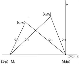
Here the problem of motion of two minor bodies with masses m₁ and m₂ is being investigated under the gravitational field of two primary bodies with masses M₁ and M₂ (M₁ ≥ M₂) moving along circular Keplerien orbits about their centre of mass where m₁ and m₂ being ≤M₂. The orbital plane is the common plane [5] . The minor bodies are taken to be attracting each other but not perturbing the primaries. To show the independence of the potential function, we shall choose our coordinate system to be rotating synodic such that two primaries are fixed on x-axis. For further simplification of the problem, we shall use dimensionless time and position variables. To find the configuration of the bodies at arbitrary equilibrium $\left(x_{i0,}{y}_{i0}\right)\left(i=1,2\right)$ a constant acceleration $a_{x_i}{x}_i,a_{y_i}{y}_i$ will be applied.

Referred to the above synodic system when the origin is taken at the smaller primary, the differential equation describing the restricted problem of three bodies may be written as:

$\begin{array}{l}{\ddot{x}}_i-2\stackrel{\dot{}}{y}=\frac{1}{{\mu }_i}\frac{\partial T}{\partial x_i}\\ {\ddot{y}}_i+2\stackrel{\dot{}}{x}=\frac{1}{{\mu }_i}\frac{\partial T}{s\partial y_i}\end{array}$ (2.1)

where, (.) denotes the differential coefficient with respect to t and

$\begin{array}{l}T={\displaystyle \underset{i=1}{\overset{2}{\sum }}{\mu }_i\left[\frac{1}{2}{\left(1-\mu +x_i\right)}^2+y_i{}^2\right]}+\frac{1-\mu }{{\delta }_{1i}}+\frac{\mu }{{\rho }_{2i}}+\frac{1}{2}\frac{{\mu }_{3-i}}{R}+a_{x_i}{x}_i+a_{y_i}{y}_i,\\ \mu =\frac{M_2}{M_1+M_2},{\mu }_i=\frac{m_i}{M_1+M_2},\\ {\delta }_{1i}^2={\left(x_i+1\right)}^2+y_i{}^2,{\rho }_{2i}^2=x_i^2+y_i^2,\\ R^2={\left(x_1-x_2\right)}^2+{\left(y_1-y_2\right)}^2,\\ l=M_1{M}_2=\text{Dimensional}\text{length}=1\left(\text{chosen}\text{as}\text{dimensionless}\right).\end{array}$

It has been examined [5] that the motion takes place in the xy-plane and so we have not considered z-coordinate.

The control acceleration for maintaining a desired equilibrium point (x_i0, y_i0) will be given as:

$\begin{array}{l}{a}_{x_{i0}}=\left(1-\mu \right)\frac{1+x_{i0}}{{\delta }_{{\left(1i\right)}_0}^3}+\mu \frac{x_{i0}}{{\rho }_{{\left(2i\right)}_0}^3}-x_{i0}+\mu -1-{\mu }_3-i\frac{\partial }{\partial x_i}\left(\frac{1}{R}\right),\\ a_{y_{i0}}=\left(1-\mu \right)\frac{y_{i0}}{{\delta }_{{\left(1i\right)}_0}^3}+\mu \frac{y_{i0}}{{\rho }_{{\left(2i\right)}_0}^3}-y_{i0}-{\mu }_3-i\frac{\partial }{\partial y_i}\left(\frac{1}{R}\right).\left(i=1,2\right)\end{array}$

In order to consider the linear stability condition we shall prefer to write the Hamiltonian with respect to the origin taken to be the equilibrium point (x_i0, y_i0), so that

$\begin{array}{l}{\xi }_i=x_i-x_{i0},{\eta }_i=y_i-y_{i0},\\ p_{{\xi }_i}=p_{x_i}-p_{x_{i0}},p_{{\eta }_i}=p_{y_i}-p_{y_{i0}}.\left(i=1,2\right)\end{array}$

where ${\xi }_i,{\eta }_i,p_{{\xi }_i}\&p_{{\eta }_i}$ are the variable in the canonic variables $x_i,y_i,p_{x_i}\&p_{y_i}$ as introduced in [10] . The corresponding Hamiltonian H may be written as:

$\begin{array}{l}\frac{1}{2}{\displaystyle \underset{i=1}{\overset{2}{\sum }}[\left(p_{{\xi }_i}^2+p_{{\eta }_i}^2\right)+p_{{\xi }_i}{\eta }_i-p_{{\xi }_i}{\eta }_i-p_{{\eta }_i}{\xi }_i+{\xi }_i\left(\mu -1-x_{i0}\right)-{\eta }_i{y}_{i0}-\frac{1-\mu }{{\delta }_{{\left(1i\right)}_0}}}\\ -\frac{\mu }{{\rho }_{{\left(2i\right)}_0}}-\frac{1}{2}\frac{{\mu }_{3-i}}{R}-a_{xi}{\xi }_i-a_{y_i}{\eta }_i]\end{array}$

$\begin{array}{l}{\delta }_{{\left(1i\right)}_0}=\sqrt{{\left(1+{\xi }_i+x_{i0}\right)}^2+{\left({\eta }_i+y_{i0}\right)}^2},\\ {\rho }_{{\left(2i\right)}_0}=\sqrt{{\left({\xi }_i+x_{i0}\right)}^2+{\left({\eta }_i+y_{i0}\right)}^2}.\end{array}$

It has been seen [5] that the motion with minor body having the mass µ₁ is independent of the motion of the minor body with mass µ₂ thus it is seen that the problem reduces to two restricted problem with µ₁ and µ₂ respectively. Taking the advantage of this conclusion our problem reduces to that studied by [10] , if we write two Hamiltonians $H\left({\mu }_1\right)$ & $H\left({\mu }_2\right)$ for $\left(x_1,y_1\right)$ & $\left(x_2,y_2\right)$ respectively. Avoiding repetitions with [10] , we may write H as:

$H=H_0+H_2\left({\mu }_1\right)+H_2\left({\mu }_2\right)$ ,

where

$H_2\left({\mu }_1\right)=\frac{1}{2}\left(p_{{\xi }_1}^2+p_{{\eta }_1}^2\right)+n\left(p_{{\xi }_1}{\eta }_1-{\xi }_1{p}_{{\eta }_1}\right)+a_1{\xi }_1^2+b_1{\xi }_1{\eta }_1+c_1{\eta }_1^2$ ,

$H_2\left({\mu }_2\right)=\frac{1}{2}\left(p_{{\xi }_2}^2+p_{{\eta }_2}^2\right)+n\left(p_{{\xi }_2}{\eta }_2-{\xi }_2{p}_{{\eta }_2}\right)+a_2{\xi }_2^2+b_2{\xi }_2{\eta }_2+c_2{\eta }_2^2$

$a_i,b_i,\&c_i$ , may be expressed as [10] with the suffix, $\left(i=1,2\right)$ along the variables $\xi ,\eta ,x_0\&y_0$ .

3. Linear Stability Condition

Thus the linearized equation of motion may be written as

${\stackrel{\dot{}}{p}}_{{\xi }_i}=-\frac{\partial H_2}{\partial {\xi }_i}=p_{{\eta }_i}-2a_i{\xi }_i-b_i{\eta }_i$ ,

${\stackrel{\dot{}}{p}}_{{\eta }_i}=-\frac{\partial H_2}{\partial {\eta }_i}=p_{{\xi }_i}-2c_i{\eta }_i-b_i{\xi }_i$ ,

${\stackrel{\dot{}}{\xi }}_i=\frac{\partial H_2}{\partial p_{{\xi }_i}}=p_{{\xi }_i}+n{\eta }_i$ (3.1)

${\stackrel{\dot{}}{\eta }}_i=\frac{\partial H_2}{\partial p_{{\eta }_i}}=p_{{\eta }_i}-n{\xi }_i$

The corresponding characteristic equation may be written as

${\lambda }^{\text{4}}+2f_i{\lambda }^2+g_i=0,\left(i=1,2\right).$ (3.2)

where $f_i=a_i+c_i+1=2\frac{{\delta }_{1i}^3-1}{2{\delta }_{1i}^3}+\mu \frac{{\rho }_{2i}^3-{\delta }_{1i}^3}{2{\rho }_{2i}^3{\delta }_{1i}^3}$

$\begin{array}{c}{g}_i=-b_i^2+2a_i\left(2c_i-1\right)-2c_i+1\\ =\frac{{\delta }_{1i}^6-2+{\delta }_{1i}^3}{{\delta }_{1i}^6}+\frac{\mu }{4{\rho }_{2i}^5{\delta }_{1i}^6}(-4{\rho }_{2i}^5{\delta }_{1i}^3+16{\rho }_{2i}^5+4{\rho }_{2i}^2{\delta }_{1i}^6+18{\delta }_{1i}^3-9{\delta }_{1i}^5\\ +2{\rho }_{2i}^2{\delta }_{1i}^3-9{\delta }_{1i}{\rho }_{2i}^4-9{\delta }_{1i})-\frac{{\mu }^2}{4{\rho }_{2i}^6{\delta }_{1i}^6}(-9{\rho }_{2i}{\delta }_{1i}^5+18{\rho }_{2i}{\delta }_{1i}^3-9{\rho }_{2i}^5{\delta }_{1i}\\ +18{\rho }_{2i}^2{\delta }_{1i}-8{\delta }_{1i}^6-9{\rho }_{2i}{\delta }_{1i}+8{\rho }_{2i}^6+2{\delta }_{1i}^3{\rho }_{2i}^3),\left(i=1,2\right)\end{array}$ (3.3)

In order to have the linear stability the following conditions are to be satisfied

$\begin{array}{l}\text{a)}{f}_i^2-g_i>0,\\ \text{b)}{f}_i>0,\left(i=1,2\right)\\ \text{c)}{g}_i>0.\end{array}$ (3.4)

4. Minimum Control Artificial Equilibrium Point

With the existence of stable region in the referred problem our next step will be to identify the stable point inside the region for which the required control acceleration is as small as possible.

In this regard our problem will be to fix the equilibrium distance ρ_(2i)0 from the second primary and to search the space craft position that provides minimum control acceleration. For this we shall minimize the objective function.

$J_i=a_{x_i}^2+a_{y_i}^2\left(i=1,2\right)$ (4.1)

$\begin{array}{l}{J}_i=\frac{\mu \left({\rho }_{2i}^3-1\right)\left({\rho }_{2i}-1\right)\left(\mu +{\rho }_{2i}^3+{\rho }_{2i}\right)}{{\rho }_{2i}^4}-\frac{1-\mu }{{\rho }_{2i}^3{\delta }_{1i}^4}\\ \times \left[\left(\mu -{\rho }_{2i}^3\right){\delta }_{1i}^6-\left(\mu -2{\rho }_{2i}^3+\mu {\rho }_{2i}^3\right){\delta }_{1i}^3+\mu \left({\rho }_{2i}^3-1\right)\left({\rho }_{2i}^2-1\right){\delta }_{1i}-\left(1-\mu \right){\rho }_{2i}^3\right].\end{array}$

which is written just by putting an index i with δ₁ & δ₂ in corresponding expressions in the referred work.

For minimum value of $J_i$ , we shall put

$\frac{\partial J_i}{\partial {\delta }_{11}}=0=\frac{\partial J_2}{\partial {\delta }_{12}}$

Where the corresponding expression as given in the referred paper may be written which we shall not write for the sake of repetition. Solving δ₁₁ & δ₁₂ by the perturbation method and restricting to µ², we have

$\begin{array}{l}{\delta }_{i\left(opt\right)}={\delta }_{1i}^{\left(0\right)}+\mu {\delta }_{1i}^{\left(1\right)}+{\mu }^2{\delta }_i^{\left(2\right)}\\ =1+\frac{1-{\rho }_{2i}^3}{6{\rho }_{2i}}\mu -\frac{{\rho }_{2i}^8+2{\rho }_{2i}^6-2{\rho }_{2i}^5+2{\rho }_{2i}^3+{\rho }_{2i}^2-4}{36{\rho }_{2i}^4},\left(i=1,2\right)\end{array}$

The corresponding control acceleration restricting to 0 (µ²) will be written as

$a_i=\sqrt{a_{x_i}^2+a_{y_i}^2}=\frac{\mu }{{\rho }_{2i}}\sqrt{1-\frac{{\rho }_{2i}^2+8{\rho }_{2i}^3-2{\rho }_{2i}^5-4{\rho }_{2i}^6+{\rho }_{2i}^8}{4}},\left(i=1,2\right)$

and the corresponding dimensional acceleration may be written as

$a_i=\frac{G{M}_2}{{\rho }_{2i}^2{l}^2}\sqrt{1-\frac{{\rho }_{2i}^2+8{\rho }_{2i}^3-2{\rho }_{2i}^5-4{\rho }_{2i}^6+{\rho }_{2i}^8}{4}}$

For an approximate analytical estimation of the distance from the second primary allowing the stability may be written as

$\begin{array}{l}{\rho }_{2i}^6-26{\rho }_{2i}^3\mu +\rho {\mu }^2\succ 0,\\ {\rho }_{2i}^3-\mu \succ 0,\\ -2{\rho }_{2i}^8+3{\rho }_{2i}^6-{\rho }_{2i}^5+8{\rho }_{2i}^3-16\mu \succ 0.\end{array}$

From the first two conditions we have

${\rho }_{2i}>{\rho }_{2i\left(\min \right)}={\left(13\mu +4\mu \sqrt{10}\right)}^{\frac{1}{3}}\approx {\left(26\mu \right)}^{\frac{1}{3}}$

and

$a\left({\rho }_{2i\left(\min \right)}\right)=\frac{{\left(26\mu \right)}^{\frac{1}{3}}\left|1-26\mu \right|\sqrt{4-{\left(26\mu \right)}^{\frac{2}{3}}}}{52}$

Finally, the minimum control acceleration will be

$\begin{array}{l}{r}_{\min }\simeq l{\left(26\mu \right)}^{\frac{1}{3}},\text{and}\\ \hat{a}\left(r_{\min }\right)\simeq \frac{G{M}_2}{\mu l^2}\left[\frac{{\left(26\mu \right)}^{\frac{1}{3}}\left|1-26\mu \right|\sqrt{4-{\left(26\mu \right)}^{\frac{2}{3}}}}{52}\right]\end{array}$

Since the expression for $r_{\min }$ & $â\left(r_{\min }\right)$ are independent of the indices (i), so they will be the expressions for both minor bodies.

5. Restricted Problem of 2 + 2 Bodies with a Primary Body of the Shape of an Oblate Spheroid

Here we shall use the notations of the work [11] . The equations of motion may be written as

$\begin{array}{l}\ddot{x}-2n{\stackrel{\dot{}}{y}}_i=\frac{1}{{\mu }_i}\frac{\partial \Gamma }{\partial x_i},\\ \ddot{y}+2n{\stackrel{\dot{}}{x}}_i=\frac{1}{{\mu }_i}\frac{\partial \Gamma }{\partial y_i}.\end{array}$ (5.1)

where

$\begin{array}{l}\Gamma ={\displaystyle \underset{i=1}{\overset{2}{\sum }}{\mu }_i}\left[\frac{1}{2}n\left\{{\left(x_i+1-\mu \right)}^2+y_i^2\right\}+\frac{1-\mu }{{\delta }_{1i}}+\frac{\mu }{{\rho }_{2i}}+\frac{\left(1-\mu \right)}{2{\delta }_{1i}^3}+\frac{1}{2}\frac{{\mu }_{3-i}}{R}+a_{x}x+a_{y}y\right],\\ \mu =\frac{M_2}{M_1+M_2}{\mu }_i=\frac{m_i}{M_1+M_2},\\ {\delta }_{1i}^2={\left(x_i+1\right)}^2+y_i^2,{\rho }_{2i}^2=x_i^2+y_i^2,R^2={\left(x_1-x_2\right)}^2+{\left(y_1-y_2\right)}^2,\\ n^2=1+\frac{3A_1}{2},A_1=\frac{R_e^2-R_p^2}{5{\bar{R}}^2}.\end{array}$

R_e = Equatorial radius of larger mass,

R_p = Polar radius of the larger mass,

$\bar{R}$ = the mutual distance between the primaries.

The Equation (5.1) may be detailed as

$\begin{array}{c}{\ddot{x}}_1-2n{\stackrel{\dot{}}{y}}_1=\frac{1}{{\mu }_1}[n^2\left(1-\mu +x_i\right)-\frac{\left(1-\mu \right)\left(1+x_i\right)}{{\delta }_{1i}^3}-\frac{\mu x_i}{{\rho }_{2i}^3}\\ -\frac{3\left(1-\mu \right)A_1\left(1+x_{1i}\right)}{2r_{11}^5}+a_{x_1}-\frac{{\mu }_2}{R^3}\left(x_1-x_2\right)]\end{array}$

${\ddot{y}}_1+2n{\stackrel{\dot{}}{x}}_1=\frac{1}{{\mu }_1}\left[n^2{y}_1-\frac{\left(1-\mu \right)y_1}{{\delta }_{1i}^3}-\frac{\mu y_i}{{\rho }_{2i}^3}-\frac{3\left(1-\mu \right)A_1{y}_1}{2{\delta }_{11}^5}+a_{y_1}-\frac{{\mu }_2}{R^3}\left(y_1-y_2\right)\right]$

$\begin{array}{c}{\ddot{x}}_2-2n{\stackrel{\dot{}}{y}}_2=\frac{1}{{\mu }_2}[n^2\left(1-\mu +x_2\right)-\frac{\left(1-\mu \right)\left(1+x_2\right)}{{\delta }_{12}^3}-\frac{\mu x_2}{{\rho }_{22}^3}\\ -\frac{3\left(1-\mu \right)A_1\left(1+x_2\right)}{{\delta }_{12}^5}+a_{x_1}-\frac{{\mu }_2}{R^3}\left(x_1-x_2\right)]\end{array}$

${\ddot{y}}_2+2n{\stackrel{\dot{}}{x}}_2=\frac{1}{{\mu }_2}\left[n^2{y}_2-\frac{\left(1-\mu \right)y_2}{{\delta }_{12}^3}-\frac{\mu y_2}{{\rho }_{22}^3}-\frac{3\left(1-\mu \right)A_1{y}_2}{2{\delta }_{12}^5}+a_{y_2}-\frac{{\mu }_2}{R^3}\left(y_2-y_1\right)\right]$

Then the equilibrium point (x₁₀, y₁₀), (x₂₀, y₂₀) will be given by

$\begin{array}{c}{a}_{x_1}=-n^2\left(1-\mu +x_1\right)+\frac{\left(1-\mu \right)\left(1+x_1\right)}{{\delta }_{11}^3}+\frac{\mu x_1}{{\rho }_{21}^3}+\frac{3\left(1-\mu \right)A_1\left(1+x_1\right)}{2{\delta }_{11}^5}\\ +\frac{{\mu }_2\left(x_1-x_2\right)}{2{\delta }_{11}^3}+\frac{{\mu }_{2\left(x_1-x_2\right)}}{R^3}\end{array}$

$a_{y_1}=-n^2{y}_1+\frac{\left(1-\mu \right)y_1}{{\delta }_{11}^3}+\frac{\mu y_1}{{\rho }_{21}^3}+\frac{3\left(1-\mu \right)A_1\left(1+x_1\right)}{{\delta }_{11}^5}+\frac{{\mu }_2\left(y_2-y_1\right)}{R^3}$

$a_{x_2}=-n^2\left(1-\mu +x_2\right)+\frac{\left(1-\mu \right)\left(1+x_2\right)}{{\delta }_{12}^3}+\frac{\mu x_2}{{\rho }_{22}^3}+\frac{3\left(1-\mu \right)\left(1+x_2\right)}{{\delta }_{12}^5}+\frac{{\mu }_1\left(x_2-x_1\right)}{R^3}$

$a_{y_2}=-n^2{y}_2+\frac{\left(1-\mu \right)y_2}{{\delta }_{12}^3}+\frac{\mu y_2}{{\rho }_{22}^3}+\frac{3\left(1-\mu \right)y_2}{{\delta }_{12}^5}+\frac{{\mu }_1\left(y_2-y_1\right)}{R^3}$

Let us take the variation in the coordinates as in the referred paper

$\begin{array}{l}{\xi }_i=x_i-x_{i0},{\eta }_i=y_i-y_{i0},\\ p_{{\xi }_i}=p_{x_i}-p_{x_{i0}},p_{{\eta }_i}=p_{y_i}-p_{y_{i0}}.\end{array}$

And the corresponding Hamiltonian may be written as

$\begin{array}{l}H=\frac{1}{2}{\displaystyle \underset{i=1}{\overset{2}{\sum }}[\left(p_{{\xi }_i}^2+p_{{\eta }_i}^2\right)+\eta \left(p_{{\xi }_i}{\eta }_i-p_{{\eta }_i}{\xi }_i\right)+n^2{\xi }_i\left(\mu -1-x_0\right)-n^2{\eta }_i{y}_0-\frac{1-\mu }{{\delta }_{1i}}-\frac{\mu }{{\rho }_{21}}}\\ \underset{}{\overset{}{\underset{}{\overset{}{}}}}-\frac{\left(1-\mu \right)A_1}{2{\delta }_{1i}^3}-\frac{1}{2}\frac{{\mu }_{3-i}}{R}-a_{x_i}{\xi }_i-a_{y_i}{\eta }_i].\end{array}$

To avoid repetition we shall after some algebraic manipulation with the addition of the extra term $-\frac{\left(1-\mu \right)A_1}{2{\delta }_{1i}^3}-\frac{1}{2}\frac{{\mu }_{3-i}}{R}$ in the Hamiltonian, we may write in dimensional units the minimum distance from the second primary as $r_{2i}^{\left(\min \right)}\approx l{\left(25\mu \right)}^{\frac{1}{3}}$ and the required dimensional control acceleration will be $a\left(r_{2i}^{(\min )}\right)=\frac{G{M}_2}{\mu l^2}\frac{\left[{\left(25\mu \right)}^{\frac{1}{3}}\left|1-25\mu \right|\sqrt{{\left|4-25\mu \right|}^{\frac{2}{3}}}\right]}{50}$ . So we find that the minimum

control acceleration is less than the one with the absence of obliquity in the shape of the primary body.

6. Conclusion

In the present work we have investigated the minimum acceleration that will put two spacecrafts at definite equilibrium position. It is concluded that the presence of a primary with the shape of an oblate spheroid decreases the thrust and it is an advantage over the case when the shape is to be spherical or the bodies are taken to be point masses. Here the two cases of the restricted problem of 2 + 2 bodies have been considered and utilizing this result established by (Whipple, 1984) for negligible masses µ₁ & µ₂, this problem has been split into two separate claimed restricted problems of three bodies and the problem reduces to that studied in the referred paper [10] and our investigation just reduces to review the work. Similarly when the shape of a primary body is taken into consideration, the conclusion reduces to that of [11] and since the results are independent of indices, so they will be the same for both the equilibrium points and this mathematical work reduces to those done in the referred paper which we have avoided and suggest that the paper should be read with the referred papers.

Conflicts of Interest

The authors declare no conflicts of interest.

References

[1]	Whipple, A.L. and Szebehely, V. (1983) The Restricted Problem of n+1 Bodies. Celestial Mechanics, 32, 137-144. https://doi.org/10.1007/BF01231121
[2]	Duboshin, G.N. (1982) On Regular Solution in the Problem of Two Rigid Bodies. Celestial Mechanics, 27, 267-284. (In French)
[3]	Duboshin, G.N. (1984) The Problem of Three Bodies. Celestial Mechanics and Dynamical Astronomy, 33, 31-47.
[4]	Milani, A. and Nobili, A.M. (1988) Instability of the 2+2 Body Problem. Celestial Mechanics, 41, 153-160. https://doi.org/10.1007/BF01238759
[5]	Whipple, A.L. (1984) Equilibrium Solutions of the Restricted Problem of 2+2 Bodies. Celestial Mechanics, 33, 271-294. https://doi.org/10.1007/BF01230509
[6]	Tsiolkovsky, K. (1936) In Extension of Man into Outer Space, 2, United Technical Press. (In Russian)
[7]	Tsander, K. (1967) From a Scientific Heritage, NASA Technical Translation TTF-541.
[8]	Mclnnes, C.R. (1999) Solar Sailing Technology, Dynamics and Mission Application. Springer-Praxis, London.
[9]	Subba Rao, P.V. and Sharma, R.K. (1997) Effect of Oblateness on the Non Linear Stability of L4 in the Restricted Three Body Problem. Celestial Mechanics and Dynamical Astronomy, 63, 291-312.
[10]	Bombardelli, C. and Peláez, J. (2011) On the Stability of Artificial Equilibrium Points in the Circular Restricted Problem of Three Bodies. Celestial Mechanics & Dynamical Astronomy, 109, 13-26. https://doi.org/10.1007/s10569-010-9317-z
[11]	Ranjana. K and Kumar, V. (2013) On the Artificial Equilibrium Points in a Generalized Restricted Problem of Three Bodies. International Journal of Astronomy and Astrophysics, 3, 508-516. https://doi.org/10.4236/ijaa.2013.34059