Numerical Solution of Nonlinear Integro-Differential Equations with Initial Conditions by Bernstein Operational Matrix of Derivative ()
1. Introduction
Some of the phenomena in physics, electronics, biology, and other applied sciences lead to nonlinear VolterraFredholm integro-differential equations. Of course, these equations can also appear when transforming a differential equation into an integral equation [1-7]. In these kinds of equations, the unknown function  appears on both sides; it appears under the integral sign on one side, while it appears as an ordinary derivative on the other side. Investigating the results of nonlinear integrodifferential equations, we observe that no obvious algebraic method has been recognized to solve these equations, and thus, approximation methods are used to solve such equations [8-10]. Bernstein polynomials (B-plynomials) have many useful properties [11,12]. In this paper, we use Bernstein polynomials and their resulting operational matrices to solve the following nonlinear VolterraFredholm integro-differential equations with the initial conditions indicated as:
 (1)
(1)
where the functions  and
and  are known, whereas
  is unknown. We approximate phrases including derivative of unknown function by operational matrix of derivative
 ; and approximate phrases including powers of unknown function by Bernstein polynomial matrix
 . This yields an equation based on the unknown
  which is the approximation
 . To examine the accuracy of the formula, we present some examples. We will show the difference between the accurate and approximation solutions in these examples upon knowing.
2. Bernstein Polynomials and Their Properties
2.1. Definition of Bernstein Polynomials Basis
The Bernstein basis polynomials of degree  are defined by:
 (2)
(2)
By using binomial expansion of , one can show that
 (3)
(3)
With the aid of Equation (3), the Bernstein vector
 (4)
(4)
can be written in the form
 (5)
(5)
where
2.2. Function Approximation
A function , square integrable in (0,1), may be expressed in terms of Bernstein basis [13]. In practice, only the first
  terms Bernstein polynomials are considered. Hence, if we write
 (7)
(7)
where
 (8)
(8)
then
 (9)
(9)
where  is said dual matrix of
  and is given in [13]. We can also approximate the function
 by double Fourier expansion as follows
 (10)
(10)
where

and  elements are given by
 (11)
(11)
for . Due of (9), we obtain
 (12)
(12)
2.3. Operational Matrix of Integration
In performing arithmetic and other operations on Bernstein basis, we frequently encounter the integration of the vector  defined in Equation (4) by
 (13)
(13)
where  is the
  operational matrix for integration and is given in [13,14].
2.4. Product Operational Matrix
It is always necessary to evaluate the product of  and
and , which is called the product matrix of Bernstein polynomials basis. Let
 (14)
(14)
Then, multiplying the matrix  with the vector
  which is defined in Equation (8), we obtain
 (15)
(15)
where  is an
is an  matrix and is called the coefficient matrix. The details of obtaining this matrix are given in [13].
3. Operational Matrix of Derivative
The differentiation of vector  in Equation (4) can be expressed as:
 (16)
(16)
where  is the
  operational matrix of derivatives for Bernstein polynomials. From (5), we have
  and then

 (17)
(17)
Defining  matrix
  and vector
  as
as
 (18)
(18)
Equation (17) may then be restated as
 (19)
(19)
We now expand vector  in terms of
 . We get
  where
where
 (20)
(20)
So
 (21)
(21)
Therefore, we have the operational matrix of derivative as
 (22)
(22)
If we approximate , then for
  (
( is the order of derivatives), we get
 (23)
(23)
4. Operational Matrices for Numerical Solution of NVFIDE
To obtain the approximate solution of the (1) under the initial conditions, the following matrix method is used. Function  is approximated by using a finite number of terms in (7) as
 (24)
(24)
The approximate functions  and
and  by Bernstein polynomials can be framed by:
 (25)
(25)
where  and
and  are defined with (12). For numerical implementation of the method explained in this section, we need to evaluate
  and
and  where
where  and
and  are positive integers, as follows
 (26)
(26)
From (14) and (16), we have
 (27)
(27)
where the vector  is an
is an  -vector;
then, for , we get
 (28)
(28)
Therefore, with this method we can approximate  and
and  arbitrary
  and
and .
.
Suppose that this method holds for  where
where
 We obtain it for
  as follows
 (29)
(29)
We have a similar relation for . So, the components of
  and
and  can be computed in terms of components of unknown vector
 . In this case, for the Volterra and Fredholm part of (1), we have
 (30)
(30)
and
 (31)
(31)
Also, to approximate the differential part of Equation (1), making use of Equation (23) we have
 (32)
(32)
After substituting the approximate Equations (24)-(32) in (1), we get
 (33)
(33)
And also, for the initial conditions, we have
 (34)
(34)
The initial conditions Equation (34) give two linear equations. Since the number of unknowns for a vector  in (33) is
 , then we collocate Equation (33) in
  Newton-Cotes points as
 (35)
(35)
For collocating Equation (33), we have used the Newton-Cotes points because of their simplicity and their good utility in our implementation as regards the speed and accuracy of answers. However, we can use other points like the Gauss points, Clenshaw-Curtis points, Lobatto points, etc. Here we present the final system:
 (36)
(36)
After solving nonlinear system (36), we get ; thenwe have the approximate solution of Equation (1).
5. Numerical Examples
To illustrate the effectiveness of the proposed method in the present paper, several examples are presented in this section.
Example 1. Consider the nonlinear Fredholm integrodifferential equation [15].
 (37)
(37)
The exact solution is . The results of proposed method for this example are exhibited in Table 1 with 4 choices of
 . For this complicate NFIDE with a small number of Bernstein basis functions, we get acceptable results.
By applying the method in Section 4, for , we have


Table 1. Approximate and exact solutions for Example 1.


We obtain the approximate solutions of the problem for  and
and  respectively,
Example 2. Consider the nonlinear Fredholm integrodifferential equation, as follows [16]:
 (38)
(38)
The exact solution is . Taking
 , we compare the obtained solution with exact solution and method [16] in Table 2.
By applying the method in Section 4, we have for ,
,

 .
.
We obtain the approximate solutions of the problem  for
for .
.
Example 3. Consider the nonlinear Volterra integrodifferential equation, as follows:
 (39)
(39)
where the exact solution is . Table 3 with 4 choices of
  illustrates the numerical results for this example.

Table 2. Approximate and exact solutions for Example 2.
By applying the method in Section 4, we have for .
.


Example 4. Consider the nonlinear Volterra-Fredholm integro-differential equation
 (40)
(40)
where 
The exact solution is . The results of proposed method on this example are exhibited in Table 4 with 4 choices of
 . For this complicated NVFIDE, we get acceptable results with a small number of Bernstein basis functions. We obtain the approximate solutions of the problem for
  and
and  respectively,


Table 3. Approximate and exact solutions for Example 3.

Table 4. Approximate and exact solutions for Example 4.
 In this regard, we have reported in figures and a table, the values of the exact solution
 , the approximate solution
 , and the absolute error function
  at the selected points of the given interval.
We have zoomed out Figures 1 and 2 to a great extent because the exact and approximate solutions are very close.
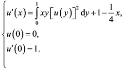
Example 5. Finally, consider the nonlinear VolterraFredholm integro-differential equation [17].
 (41)
(41)
where, .
.
The exact solution is . The results of the proposed method for this example are exhibited in Table 5 with 4 choices of
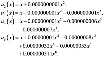
 . For this complicated NVFIDE, we get acceptable results with a small number of Bernstein basis functions. We obtain the approximate solutions of the problem for
  and
and  respectively,


In this regard, we have reported in figures and a table, the values of the exact solution , the approximate solution
 , and the absolute error function
 at the selected points of the given interval.

Figure 1. Comparison of the exact solution and the approximate solutions for Example 5.

Figure 2. Comparison of the absolute error functions for Example 5.

Table 5. Approximate and exact solutions for Example 5.

Figure 3. Comparison of the exact solution and the approximate solutions for Example 5.

Figure 4. Comparison of the absolute error functions for Example 5.
We have zoomed out Figures 3 and 4 to a great extent because the exact and approximate solutions are very close. While in [17], the adopted method yields no solution for , takes time to give the approximate answer for
 , and is proper only for
 , our method is significant not only because it yeilds solutions for any n, but also because the approximate solutions it gives are very close to exact ones.
6. Conclusion
In this paper, we have proposed a numerical solution to solve nonlinear Volterra-Fredholm integro-differential equations with initial condition by Bernstein polynomials operational matrices and derived operational matrix. We use formula for numerical examples and it is obvious that the numerical solution coincides with the exact solution even with a few Bernstein polynomials used in the approximation. Finally, errors show that the approximation becomes more accurate when n is increased. Therefore, for better results, it is recommended to use a larger n.