1. Introduction
The owner-occupied residence is an important element in portfolio of the average household. The traditional financial justifications for home ownership are that the household can take advantage of the income tax provisions that permit deductions for interest and property taxes, paying down the home loan is a form of forced saving that builds wealth, and ownership is a good hedge against inflation. Indeed, Kain and Quigley [1] pointed out that restrictions on home ownership faced by minority households put them at a severe financial disadvantage. The sharp up and down movements in housing prices in the past 15 years have called the financial advantage of home ownership into question. A study by Pfeffer as reported by Bernasek [2] found that the real wealth of the median household (2013 dollars) fell from $87,992 in 2003 to $56,355 in 2013, largely because of the decline in housing prices.
Hypothesized causes of the housing price bubble that led to the financial crisis and deep recession of 2007- 2009 fall into four categories. One blames the financial system with its unsound lending practices, complex mortgage-backed securities, and the shadow banking system that relied heavily on high degrees of financial leverage and short-term borrowing. Another places blame on the federal government and the Federal Reserve Bank through aggressive deregulation (and failure to implement existing regulations), monetary policy that held the federal funds rate at very low levels during the critical years of 2001-2004, and aggressive policies to increase home ownership. A third view points to a flood of capital from abroad that resulted from a large trade deficit, and the fourth simply blames a classic asset price bubble (and inevitable crash) that is thought to have begun in the late 1990s. Each of these points of view has its adherents. Nearly all observers agree that the unsound financial system played a major role. However, those who place primary blame on the asset price bubble thought that the unsound practices of the financial system were a reaction to the asset price bubble, not the cause. Nobel-laureate Robert Shiller [3] is the most prominent member of this group, but he agreed that the interest rate policy of the Fed and the unsound practices of the financial system enhanced the housing price bubble. Taylor [4] laid much responsibility on federal policy, especially the failure to follow the Taylor Rule in setting the federal funds rate. McDonald and Stokes [5] [6] conducted empirical studies using monthly data and found that the federal funds rate was a cause of the housing price bubble.
Former officials of the Federal Reserve believed that monetary policy played little or no role in creating and sustaining the housing price bubble. Former Chairman of the Federal Reserve Benjamin Bernanke ([7] , p. 52) stated, “…the evidence I have seen suggests that monetary policy did not play an important role in raising house prices during the upswing.” He based his view in part on a study by Dokko, et al. [8] , and cited four reasons: comparisons with other nations showed that their housing price bubbles occurred with tighter monetary policies; changes in interest rates that were small in comparison to the increases in housing prices; capital inflows from emerging-market nations in search of safe investments; and (in agreement with Shiller) the fact that the price bubble may have begun before the sharp reduction in the federal funds rate. Former Vice Chair Alan Blinder ([9] , p. 38-39) agreed with Chairman Bernanke’s points, and added that the housing price bubble continued for two years after the Federal Reserve began to increase the federal funds rate in June 2004. And former Chairman Alan Greenspan [10] looked at the data for 2002-2005 and concluded that long-term rates started to fall six months before the Fed began to lower the federal funds rate in 2001, and long-term rates continued to fall after the Fed began to raise the federal funds rate in 2004. Greenspan ([10] , p. 237) stated, “But the fixed-rate mortgage clearly delinked from the federal funds rate in the early part of this century. The correlation between them fell to an insignificant 0.10 during 2002-2005, the period when the bubble was most intense, and as a consequence, the funds rate exhibited little, if any, influence on home prices.” Time-series analysis for a longer time period by McDonald and Stokes [11] showed that the interest rate on the standard 30-year mortgage was driven by the federal funds rate, and that this mortgage rate was not a cause of the housing price bubble.
Richard Grossman [12] added a fifth hypothesis-fiscal policy. He pointed out ([12] , p. 141), “The business cycle expansion that began in 2001 was given a substantial boost by a series of three tax cuts during the first three years of the administration of President George W. Bush.” Tax rates were reduced in all brackets, taxes were cut for capital gains and some dividends, and a variety of exemptions, deductions, and credits were increased. On the expenditure side, the wars in Afghanistan and Iraq added significantly to spending by the Department of Defense. Grossman agreed that unsound financial practices by the private sector and by Fannie Mae and Freddie Mac shared in the blame, but concluded ([12] , p. 151), “Nevertheless, the bulk of the blame for the crisis must be assigned to the Bush administration’s fiscal policy and the Greenspan Fed’s monetary policy.” Grossman believed that these policies were driven by ideology rather than by careful analysis.
Some of these ideas can be tested using monthly data. The purpose of this paper is to expand our earlier tests to include fiscal policy, the interest rate on adjustable-rate mortgages (as an indicator of loose lending practices), and net flows of capital from abroad. The models of housing prices in this paper also include the federal funds rate, the foreclosure rate, the unemployment rate, and the interest rate on the standard 30-year mortgage. As such, this study provides a reasonably complete test of alternative hypotheses.
In the present paper, it is argued that the variable rate mortgage, not the 30-year mortgage rate, may be the appropriate variable to use in the analysis. Buyers wishing to profit by the increases in housing prices in the pre- 2007 period most likely would be expected to hold their property for a relatively short period, and thus might have been interested in a variable rate mortgage because of the lower up-front costs rather than a fixed 30-year mortgage. When the housing prices started to get soft, and a quick turn over of the property was not realized, the owner would have been put in further financial stress when the adjustable mortgage rate moved up. These factors suggest the variable rate mortgage should be considered in place of the more traditional 30-year mortgage rate. For example, Zandi ([13] , p. 38) showed that 91% of subprime mortgages securitized in 2006 were adjustable rate loans. A majority of these loans (51%) were no-doc or low-doc loans. Alt-A loans that were securitized were 69% adjustable rate loans and 82% were no-doc or low-doc. These are the loans that were most likely to default and lead to foreclosures and large declines in the values of mortgage-backed securities. See Jiang, et al. [14] for an analysis of low-doc loans and delinquency. Other variables missing from prior models include controlling for fiscal policy (using the federal deficit as a proxy) and a measure of the net capital inflow, as measured by the Treasury Department TIC data. Both these latter variables are postulated to have a possible effect on aggregate demand in the housing market and can be thought of as controls that are needed to be added to the analysis so that the coefficients on the interest rate variables are not impacted by a possible omitted variable bias. The TIC data include net acquisitions of financial assets, but do not include direct purchases of physical assets. A description of the data is provided in the next section, which is followed by a review of previous research and models to be estimated. The empirical results are presented next, and the final section concludes.
2. Data
The study employs monthly data from January 2000 to August 2010. The housing price series is the S&P/Case- Shiller ten-city composite index. The nominal price index (not adjusted for inflation) is used because borrowers took the loans in nominal terms and defaulted in nominal terms. The federal funds rate is the actual rate recorded on the last Friday of the month in question. The fiscal policy variable is the federal government deficit for the month as provided by the U.S. Department of the Treasury. The unemployment rate for the month is from the U.S. Bureau of Labor Statistics. The Zillow foreclosure rate for the nation is a weighted average of the current and past two months for the percentage of all homes foreclosed on in the given month (with the heaviest weight on the most recent month). Foreclosures include those sold at a sheriff’s sale or forfeited to the bank. The study includes the interest rate on standard fixed payment 30-year mortgages provided by the Federal Home Loan Bank. In addition, the initial interest rate on one-year adjustable rate mortgages as provided by the Freddie Mac Primary Mortgage Market Survey is employed to capture conditions in the newer, non-standard portion of the mortgage market. The net international capital flow variable is provided by the monthly U.S. Department of the Treasury TIC survey.
Table 1 lists variable means for the raw and logged values of the monthly data on the variables used in this
![]()
Table 1. Data description for period 2000/1 to 2010/8.
Notes: For further data information see text. DF is the augmented Dickey Fuller t-test with an intercept and fixed lag = 7. Critical values for 99%, 95% and 90% are respectively −3.485, −2.885 and −2.579. The series CURR_ACT and DEFICT have been scaled by 100 and 1000 respectively.
study. In addition to mean, standard deviation and maximum/minimum values, Dickey-Fuller unit root tests are reported. If series cannot reject a unit root, yet the residuals of a vector auto-regression (VAR) model do not contain a unit root, the series in the model can be thought of as co-integrated. The new capital inflow variable proved not to be significant in any model and has been reported in only one set of results in this paper. Note that the mean for the federal funds rate is 2.76 percent, compared to 6.19 percent for the 30-year mortgage and 4.99 percent for the one-year adjustable rate mortgage. The mean monthly deficit for the federal government is $34.5 billion. The mean of the foreclosure rate is 0.036 percent, a small number. But recall that this refers to the foreclosures for just a month. And note that the minimum and maximum values for this variable are 0.011 and 0.104, a change of almost ten times!
Plots of the variables are presented in Figure 1. The S&P Case-Shiller home price index starts at 100 in January 2000, rises to 226.29 in 2006, and falls to the 160 neighborhood in 2009.
3. Discussion of Prior Research, Questions to Be Addressed and Models Used
McDonald-Stokes [5] , which was published on-line June 18, 2011, presented evidence that the Federal Reserve federal funds rate policy had an impact on the housing bubble as measured by the S&P/Case-Shiller housing price index. The study employed VAR modeling techniques using monthly data for the United States together with disaggregate models for 20 individual metro areas in the period 1987 to 2010/8. The analysis used two series, the log S&P/Case-Shiller housing price series and the log federal funds rate since that was the channel suggested by Bernanke-Binder [15] . McDonald-Stokes [6] , responding to suggestions on that paper, added the log 30-year mortgage rate, the log foreclosure rate and the log unemployment rate and again found that the shocks to the federal funds rate continued to be causally prior to movements to the S&P/Case-Shiller housing price series. In this model, shocks to the log 30-year mortgage rates did not map to the log housing price series. Positive shocks to the log unemployment rate and the log foreclosure rate did in fact have negative effects on the log housing price as would be suggested by theory. An important finding of the paper was that the effect of shocks in the log federal funds rate continued to have a significant effect on the log housing price series with the addition of these controls for alternative channels of influence.
McDonald-Stokes [16] used both aggregate and disaggregate data for 20 metro areas to estimate a model testing the effect of both the log federal funds rate and the foreclosure rate on the log housing price series using all level and difference models. The difference models were estimated to remove the low frequency information in the series and focused more on the higher frequencies. The addition of the foreclosure rate did not alter the findings concerning the effect of the federal funds rate on the log housing price series found in the McDonald-
Stokes [5] [6] . The foreclosure rate was found to interact with housing prices: a larger foreclosure rate led to lower housing prices, and lower housing prices produced a greater foreclosure rate.
Miles [17] took issue with the McDonald-Stokes’ [5] finding that shocks in federal funds were causally prior to logs of the housing price series. In Miles’ view, the shocks to the 30-year mortgage rate were what impacted the Case-Shiller price series. A major limitation of Miles’ model specification was that, when modeling the effect on the log housing price of lags of the 30-year mortgage rate, he neglected to control for lags of the log housing price on the right-hand side of the equation. As specified, he was not estimating Granger [18] causality. McDonald-Stokes [11] investigated his claim in a number of ways. First they used a VAR model, not a distributed lag model. Next they investigated whether smoothing the series using the Christiano and Fitzgerald [19] filter, which Miles suggested, or the alternative Hodrick-Prescott [20] filter to remove low frequency (long run) information would significantly impact the results. McDonald-Stokes [11] found that the results differed pending on whether filtered data or non-filtered data were used, depending on the number of lags in the VAR, and most importantly, whether lags of the left-hand side variable were in the model on the right-hand side. Miles’ results could be replicated only when using his functional form that did not have lags of the left-hand side variable on the right.
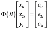
The VAR model is the basic research tool used in this paper. Its essence can be seen by assuming a three variable system  where
where  is the focus variable. The VAR model estimates
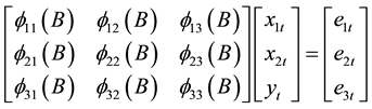
 (1)
(1)
which can be written as
 (2)
(2)
Granger causality from  to
to  implies that
  where
where  is a polynomial in the lag operator
  with
with  terms where
 . Equation 2 allows for feedback, which is not possible in an OLS or distributed lag model. A VAR model can be transformed to a VMA model, given
  is invertible, or
 (3)
(3)
where . The terms in
 ![]() measure the dynamic responses of each of the potentially endogenous variables to a shock to the system. Equation 3 can be expanded to
measure the dynamic responses of each of the potentially endogenous variables to a shock to the system. Equation 3 can be expanded to
![]() (4)
(4)
Define ![]() as the covariance of the innovations
as the covariance of the innovations![]() . Off diagonal terms are consistent with zero period relationships between the variables. To identify the model, restrictions need to be placed on
. Off diagonal terms are consistent with zero period relationships between the variables. To identify the model, restrictions need to be placed on![]() . In the current paper the usual Choleski decomposition has been used to othogonalize
. In the current paper the usual Choleski decomposition has been used to othogonalize ![]() where
where ![]() is lower triangular with positive elements on the diagonal. The Choleski decomposition imposes a semi-structural interpretation on the estimated model by transforming
is lower triangular with positive elements on the diagonal. The Choleski decomposition imposes a semi-structural interpretation on the estimated model by transforming![]() , the VMA form of the model, and thus identifies the model, given the ordering of the variables. As discussed by Enders ([21] , p. 292), in the Choleski decomposition it is assumed that an innovation in one variable does not have a contemporaneous effect on the other variables. If
, the VMA form of the model, and thus identifies the model, given the ordering of the variables. As discussed by Enders ([21] , p. 292), in the Choleski decomposition it is assumed that an innovation in one variable does not have a contemporaneous effect on the other variables. If ![]() was close to a diagonal matrix initially, which would be the case when there was no contemporaneous relationship between the residuals, the Choleski transformation would not be as important. The ordering of the variables might make a difference if
was close to a diagonal matrix initially, which would be the case when there was no contemporaneous relationship between the residuals, the Choleski transformation would not be as important. The ordering of the variables might make a difference if ![]() is not diagonal. This possibility was tested and found to make no difference in the nature of the results. The order of the variables used in the reported results is based on past findings―interest rates first, foreclosure rate next, followed by the unemployment rate, the federal deficit, capital inflow, and the lagged value of the housing price variable.
is not diagonal. This possibility was tested and found to make no difference in the nature of the results. The order of the variables used in the reported results is based on past findings―interest rates first, foreclosure rate next, followed by the unemployment rate, the federal deficit, capital inflow, and the lagged value of the housing price variable.
Significance bounds on the VMA coefficients can be obtained using Monte Carlo integration. Rats software Pro version 8.3 routine @mcgraphirf, Doan ([22] , p. 495), is used to calculate using Monte Carlo integration 95% bounds for ![]() for all the nine possible cases of the sample 3 variable VAR model. Sims and Zha [23] provide a detailed discussion of alternative methods for obtaining VMA coefficient bounds. An advantage of their suggested method, which has been used in this research, is that the estimated confidence bounds of the VMA form of the model are not assumed to be symmetric, as would be the case if bootstrap methods were attempted. An additional advantage of Monte Carlo integration is that it does not suffer from bias amplification that can occur with bootstrap methods, as noted by Sims and Zha ([23] , p. 1125).
for all the nine possible cases of the sample 3 variable VAR model. Sims and Zha [23] provide a detailed discussion of alternative methods for obtaining VMA coefficient bounds. An advantage of their suggested method, which has been used in this research, is that the estimated confidence bounds of the VMA form of the model are not assumed to be symmetric, as would be the case if bootstrap methods were attempted. An additional advantage of Monte Carlo integration is that it does not suffer from bias amplification that can occur with bootstrap methods, as noted by Sims and Zha ([23] , p. 1125).
In general, the number of lags in the VAR model m is not the number of lags in![]() , which we will call
, which we will call![]() . In the results reported later, both
. In the results reported later, both ![]() and
and ![]() were used. The lag length
were used. The lag length ![]() was selected using both the M-statistic suggested by Tiao-Box [24] and inspection of the cross correlations. B34S version 8.11F was been used to calculate these tests reported in the paper. As an example to aid interpretation, if
was selected using both the M-statistic suggested by Tiao-Box [24] and inspection of the cross correlations. B34S version 8.11F was been used to calculate these tests reported in the paper. As an example to aid interpretation, if ![]() is the log of the federal funds rate,
is the log of the federal funds rate, ![]() is the 30-year mortgage rate and
is the 30-year mortgage rate and ![]() is the log of the housing price series, the term
is the log of the housing price series, the term![]() , suitably transformed by the Choleski factorization, measures the effect of shocks in the log federal funds market on the log housing price and
, suitably transformed by the Choleski factorization, measures the effect of shocks in the log federal funds market on the log housing price and ![]() measures the effect of shocks in the mortgage market on the log housing price index. If
measures the effect of shocks in the mortgage market on the log housing price index. If ![]() for
for![]() , then each endogenous variable is not impacted from shocks coming from the other endogenous variables. In addition of graphs of impulse response function terms
, then each endogenous variable is not impacted from shocks coming from the other endogenous variables. In addition of graphs of impulse response function terms ![]() the variance of the focus variable, the log housing price can be decomposed to assess the effect of shocks from the other series by lag length.
the variance of the focus variable, the log housing price can be decomposed to assess the effect of shocks from the other series by lag length.
4. Empirical Results
The spectrums of the raw and differenced series are shown in Figure 2. The effect of differencing on removing the low frequencies in the series is shown clearly. Such a transformation will remove any unit root information but changes the interpretation of any estimated model. If all effects among the series are not at the long run (low frequency range), such a transformation will not impact the results.
Table 2 shows Granger [18] tests for three models. The first contained the log of the 30 year mortgage series; in model 2 the log of the adjustable rate series replaces the 30-year mortgage rate. All series were differenced in model 3 to remove the low frequency information. Note first that the log federal funds rate is highly significant in all models with significance values of 0.9968, 0.9984 and 0.9985. In model 1 the log 30-year mortgage rate is
![]()
Figure 2. Spectrums of the raw and differenced series.
![]()
Table 2. Granger causality tests of three VAR(7) models predicting log Case-Shiller price series.
Notes: Only the results for the equation predicting the log Case-Shiller Series are shown. Seven lags were used in the VAR. Model 1 uses the Log_Mort30 variable. Model 2 uses the Log ARM rate variable. Model 3 is the same as Model 2 except all series have been differenced. See Table 1 for variable descriptions. The top number is the F(7,78) test statistic for Models 1 and 2. For Model 3 it is F(7,77). The value in ( ) is the significance.
not significant. However, in model 2 and model 3 with the log of the adjustable rate mortgage included in raw (model 2) and differenced (model 3) form, the significance for the mortgage rate variable rises from the 0.3351 found with model 1 to 0.9618 and 0.9772 respectively. This is an important finding that supports the theoretical conjecture that the adjustable rate mortgage, not the 30-year mortgage rate, was the important variable. The significance of the log federal funds rate indicates that the mortgage rate was not the only rate to consider. The deficit is not significant in any of the models considered. The log foreclosure is significant in models 1 and 2, with values of 0.9856 and 0.9806 respectively that includes long run influences, but is not significant when the long run (low frequency) effects are removed by differencing in model 3, where it falls to 0.7168. The log unemployment variable is significant in model 2 at 0.9729. However, this significance falls to 0.9053 when we remove the long run (low frequency) information from the data series in model 3.
In order to determine the effect of the capital flow variable on the results, an expanded model 3 including the capital flow variable was estimated over a consistent dataset with 7 observations dropped. Note that unlike model 3, the deficit variable is not differenced preserving the low frequency information. The results are shown in Table 3. Note that the difference in the federal funds rate is highly significant. The difference in the adjustable rate mortgage is significant at 0.95 for lags 4 - 6, falling to 0.94 when the expanded model used 7 lags. Unlike models 1 - 3, the deficit is always significant, and the capital flow variable is not significant.
Figure 3 shows graphically the impulse response functions for model 1. The bottom row displays the responses of the Case-Shiller housing prices; the log of the federal funds rate is significant, the log 30-year mortgage rate is not significant, and the foreclosure rate and unemployment rate are significant. The federal deficit is not significant. The 30-year mortgage rate was affected positively by shocks to the federal funds rate, and by its own prior shocks. The response of the housing price to itself is strongly positive and significant, controlling for all of the variables in the model. This finding is suggestive (but not conclusive evidence) of a housing price bubble. Housing prices had significant effects on the federal funds rate and the foreclosure rate. Evidently the Federal Reserve did respond to high housing prices by increasing the federal funds rate, as shown in Figure 1. The results for housing prices and the foreclosure rate demonstrate the interaction between these two variables. The variance composition of this model listed in Table 4 shows that the effect of the federal funds rate in general has an impact after 10 months. The effect of the foreclosure rate increases continuously.
Impulse response functions for model 2 are displayed in Figure 4. In this model the rate on the one-year rate on adjustable-rate mortgages replaces the rate for the 30-year mortgage. The significant effect of the adjustable mortgage rate in model 2 is clear. The adjustable mortgage rate starts impacting housing prices in period 1, and this interest rate is not affected by shocks to the federal funds rate (in contrast to the 30-year mortgage rate). The adjustable rate mortgage variable is adding new information not provided by the 30-year mortgage variable. In model 2 the federal deficit variable almost reaches significance. As in model 1, the effects of shocks to the housing price variable are found to affect the federal funds rate and the foreclosure rate. The variance decomposition of this model shows the relative effects. Both the federal funds rate and the foreclosure rate variables are significant in model 2. The variance decomposition for model 2 in Table 5 shows that effects of the federal funds rate and the ARM rate occur within a few months after their shocks.
![]()
Table 3. Granger tests for expanded 7 variable housing price model for lags 4 to 7.
![]()
Table 4. Variance decomposition for model 1 (Decomposition of variance for series LN_CSXR).
Model 3 employs the first differences of all the series in model 2. As shown in Figure 5, once the low frequency information is removed, only shocks to the change in the federal funds rate and the change in housing prices have an impact on the change in housing prices. As shown in variance decomposition in Table 6, the difference in the federal funds rate starts having a significant effect at lag 9 that persists.
The final model in the paper includes first differences of the state variables, but does not employ first differ-
![]()
Table 5. Variance decomposition for model 2 (Decomposition of Variance for Series LOG_CSXR).
![]()
Figure 3. Impulse response functions for model 1.
![]()
Figure 4. Impulse response functions for model 2.
![]()
Figure 5. Impulse response functions for model 3.
ences of the flow variables. This treatment of the flow variables may be more appropriate in that the flow is measuring a change in a stock. The capital flow variable is included in this model. Model 4 differences log housing prices, log foreclosure rate, both log interest rates, and the log unemployment rate to remove long run effects while leaving the deficit and the capital flow un-differenced to see how this impacts the variance decomposition. The impulse response functions in Figure 6 show that shocks to changes in the federal funds rate, the ARM rate, and the foreclosure rate impact changes in housing prices. The new result is that shocks to the deficit variable (i.e., a change in federal debt) have a significant effect on changes in housing prices. The capital flow variable does not have a significant effect on the change in housing prices. The variance decomposition results in Table 7 show a sizable impact of the federal deficit. These findings must be tempered by the fact that they might be upwardly biased due to the fact that the long run (low frequency) impacts of the interest rate series and unemployment have been removed.
![]()
Figure 6. Impulse response functions for model 4 using 5 lags.
![]()
Table 6. Variance decomposition for model 3 (Decomposition of Variance for Series DLN_CSXR).
![]()
Table 7. Variance decomposition for a 5 lag extended VAR model (Decomposition of Variance for Series DLN_CSXR).
5. Conclusions
The most important finding of this study is that both the log federal funds rate and the log adjustable rate mortgage have important impacts on the log Case-Shiller housing price series. This funding is robust to specifications that include the log foreclosure rate, the log unemployment rate, and the federal deficit, which experimented with un-differenced and differenced data. The federal deficit is also found to influence housing prices in the expected direction. The net capital flow variable, also modeled as a possible source of aggregate demand in the housing sector, proved not to have had a significant effect on housing prices. This result for the capital flow variable may come as a surprise. However, the literature on asset prices and the foreign trade balance actually reverses the causation. According to Adams, et al. [25] , Gete [26] , and Laibson and Mollerstrom [27] , the large increase in housing prices that resulted in part from low interest rates led to reductions in savings and larger deficits in the current account. However, shocks to changes in housing prices had no effect on net capital flows in model 4 (Figure 6).
Much recent research has focused on testing for a bubble in the housing market unrelated to fundamental factors. Bredthauer and Geppert [28] found that, in the period 1931 to 2009, the bubble hypothesis could not be supported. On the other hand, Nneji, Brooks, and Ward [29] and Jin, Soydemir, and Tidwell [30] did find evidence of a bubble in the post-2000 period. We are agnostic on this point, and test alternative hypotheses for movements in housing prices that have been proposed.
This test of alternative hypotheses has confirmed that both monetary policy and federal fiscal policy were causes of the large increase and subsequent crash in nominal housing prices. The interest rate on adjustable rate mortgages, and not the rate on standard 30-year mortgages, also was a cause of the housing price movements. In addition, this study confirmed the earlier finding that the foreclosure rate and the housing price interacted so that foreclosures led to housing price declination, which led to more foreclosures, and so on. Shocks to housing prices affect housing prices positively in all of the estimated models. Lastly, the net capital flows from abroad are not found to have an effect on housing prices.
Acknowledgements
The authors thank participants at seminars at the University of Illinois at Chicago and attendees at sessions of the Illinois Economic Association for helpful comments.