Coupled Electromagnetic Circuits and Their Connection to Quantum Mechanical Resonance Interactions and Biorhythms ()
1. Introduction
The description of molecular processes and the energy/ charge transport in/between molecules as mechanical (and more promising) electrical oscillators has a long history [1,2]. Thus a molecule (or interacting molecules via H bond incorporating an exchange of protons) can be regarded as a certain charge distribution of proper capacitances, whereas certain molecular changes of the configurations are connected by currents. In the early quantum mechanics, Heisenberg used calculations of currents to treat transitions between ground and excited states of atoms to explain their spectral properties. These transitions usually are very fast processes (the lifetime of excited singlet states amounts to 10−7 sec; only the lifetime of excited triplet states may vary from 10−2 sec to minutes and hours). The oscillations of between molecule sites (IR spectra) are much slower (usually a factor 10−3 - 10−4 compared to singlet excitations), but are still faster compared to some biorhythms in cells. It appears that the basic principle of coupled electric oscillators is also useful to study physiological processes for many reasons: it is possible to regard cells as complex systems of charged layers/structures, and all biomolecules are usually highly charged ions (i.e. multipoles). Then it is a consequence to consider cellular systems as numerous different charge distributions (capacitances) and currents, induced by charge transfer via H bonds or other molecular deformations. This connection indicates that the origin of biochemical resonances is of quantum mechanical nature, since only this tool can determine molecular properties and resonance interactions. In recent time, the development of molecular electronics appears to be very outstanding devises [3-5]. A further interesting feature is the study of biorhythms. It is one goal of this study to show that biorhythms result from very complicated couplings of electromagnetic oscillators and by splitting of resonance frequencies. By that, we can obtain fast oscillations and, in addition, one or two frequencies, which are rather slow. In a certain sense, this result may be regarded as superimposition of beats to accelerate oscillator frequencies. Already two coupled electric oscillators are sufficient to study such a model.
2. Methods—Theoretical Part
2.1. Denominations, Abbreviations and Basic Equations
In the following, we make use of the definitions: L: inductivitance; C: capacitance; M: mutual inductivitance between two solenoids; U: voltage; Q: electric charge at the capacitance; Q∙ = dQ/dt: electric current in the solenoid; Q∙∙: second time derivative; indices refer to the related oscillator number.
The basic equation of all electromagnetic processes is the following equation:
 (1)
(1)
A further basic equation is the consideration of one electric oscillator with L and C (Figure 1(a)). From Equation (1) follows:
 (2)
(2)
The solution of Equation (2) is simply given by the “ansatz”:
 (3)
(3)
It is the task of the following sections to reduce coupled electromagnetic circuits to Equation (2) and its solution (3) via the concept of normal modes. Replacing cos(ω0t) by sin(ω0t) or by forming either a linear combination of sine and cosine or exp (iω0t), Equation (2) is also satisfied.
2.2. Coupling of Two/Three Identical Electric Oscillators: Magnetic Coupling via M (Coupling Constant) and a Qualitative Connection Tochronobiology
Thus for simplicity we first consider Figures 1(b) and 2. The basic equations applicable to both figures are:
 (4)
(4)
Without any restriction Equation (4) refers to Figure 2, whereas Figure 1(b) is described, if the connection of oscillators 1 and 2 to oscillator 3 is quenched by putting M = 0. Then oscillator 3 is completely independent (Q3 = Q) and is treated by Equations (2) and (3). For this case the normal modes are readily obtained by the substitutions:
 (5)
(5)
The solutions resulting from Equation (5) are identical with those of Equation (2), if the normal modes q1 and q2 are inserted:
 (6)
(6)
 (7)
(7)
The arbitrary amplitudes can be fixed by proper initial conditions. By taking M → 0 the connection between the oscillators is removed and ω1 = ω2 = ω0 is valid. The normal modes of 3 coupled oscillators (Figure 2) are obtained by the substitutions:
 (8)
(8)
The solutions in terms of normal modes are:
 (9)
(9)
 (10)
(10)
 (11)
(11)
Obviously the solutions (9)-(11) agree with the solution (3), if M → 0 is carried out.
 (a) (b)
Figure 1. (a) One single oscillator; (b) Two identical oscillators.

Figure 2. Extension to three identical oscillators according to Figure 1(b) with couplings between each oscillator.
Pendular Movements—Their Implications to Biorhythms and Chronobiology
Due to the coupling M the resonance frequency ω1 according to Equations (6), (7), (9) and (11) the frequencies resulting from L + M or L + 2M in the denominator can be reduced, whereas according to (7), where the difference L − M enters the denominator; ω2 may become very high, if M amounts approximately to L. Example: We choose L = C = 1 in such units that ω0 = 1 and T = 2π days (ca. 6.28 days). Please note that the definition ω = 2πT holds. Then if M = 0.9 L = 0.9 formula (7) provides T1 ≈ ca. 8.5 days and (6) T2 ≈ 0.3·2π, ca. 2 days. However, if M = 0.99 L, then there is no significant change in formula (6), i.e. T ≈ ca. 8.5 days, but formula (7b) provides T2 = 0.6 days. A sudden change of L or C may imply significant changes in the related resonance frequencies. In particular, the denominator of formula (7), where the difference L − M has to be used, may lead to severe changes of the eigenfrequency ω2 and T2. It follows that the resonance frequencies ω2 = ω3 are degenerate, and only ω1 is changed; the denominator L + 2M is increased. This provides a decrease of the eigenfrequency ω1 and a corresponding prolongation of the resonance time T1. Using again the above values C = 1, L = 1 and M = 0.99·L, then T1 amounts to ca. 11 days. In other words: Assume that the unperturbed oscillator shows a circasemi-septan period, then the feed-sideward coupled oscillators (each oscillator couples with 2 other oscillators) may lead to a circaseptan period, if the feed-sideward coupling is strong, as assumed in the above case. The solutions (6) and (7) result from two coupled oscillators and both charge amplitudes q1 and q2 linearly depend on Q1 and Q2. We may perform linear combinations of either solution (6) or (7) in order to view the amount of information containing in coupled oscillators. We show this amount in the case of solution (6) and (7). We make use of a trigonometric theorem and of the substitutions:
 (12)
(12)
Then Equations (6) and (7) can be rewritten in the form:
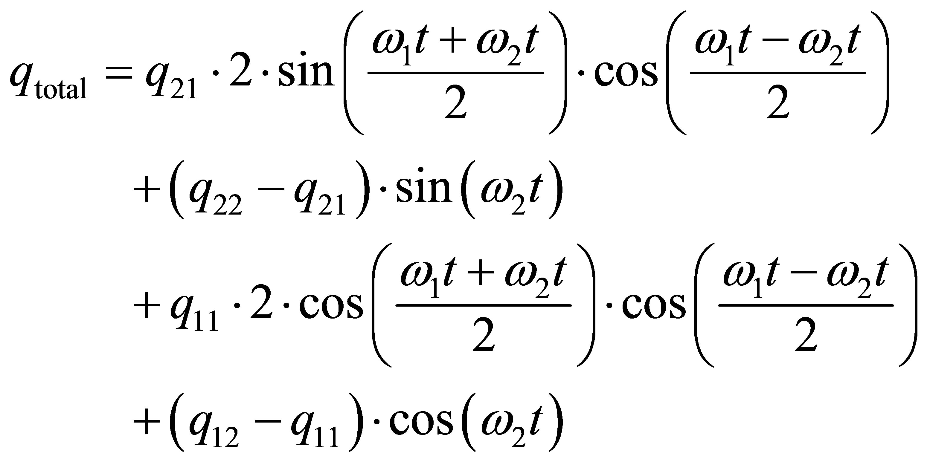 (13)
(13)
Equation (13) provides the information that the superposition amplitude qtotal contains the basic amplitudes, which are the differences q22 – q21 and q12 – q21 and the frequency ω2, a very fast oscillation frequency
 in the sine/cosine, and a very slow oscillation frequency
  in the cosine (or 2∙π/T'). If q22 = q21 and q12 = q11, the second terms of Equation (9) vanishes and the cosine is referred to as carrier amplitude/frequency incorporating “beats” between the two coupled oscillators. However, if the amplitudes q11 and q12, q22 and q21, considerably differ from each other, then beats are still present, but they do not play the main role. It appears that in chronobiology we have to deal with similar situations, where many fast oscillations simultaneously appear besides very slow oscillating components. Since the starting point of Equation (13) are two identical oscillators with one coupling M between them (this is rather a model than a very realistic case) it is evident that superpositions of more complex conditions lead to many fast oscillations and more than one beat amplitude.
2.3. Two Oscillators with L1, C1, L2, C2, a Common Dielectric Medium ε and the Coupling λ(ε)
It appears that Figure 3 represents also significant information with respect to cellular processes, since a dielectric medium between biomolecules (e.g. water) is rather realistic. The presence of any dielectric medium in a capacitance C may also change its magnitude. The basic equations according to Figure 3 are:
 (14)
(14)
The solution procedure is the same as already used:
 (15)
(15)
This “ansatz” provides the matrix equation:
 (16)
(16)
The perturbed eigenfrequencies of the electrically coupled oscillators are given by:
 (17)
(17)
If the connection via a proper dielectric medium is vanishing (λ → 0), we obtain two isolated systems. It should be mentioned that with the help of the frequencies ω1 and ω2 we are able to form again two different linear combinations in terms of cosine/sine, and pendular movements according to the solution (13) follow from this behavior. This problem will be discussed in connection with the next section.
2.4. Magnetic Coupling between 3 Different Oscillators
The problem is solved similar to Equation (4). Instead of unique parameters M, L, C we now consider the case (Figure 4) L1, C1, L2, C2, M12 = M21, L3, C3, M13 = M31, M23 = M32:
 (18)
(18)
The eigenfrequencies of the uncoupled oscillators are:
 (19)
(19)
Equation (18) is solved in the same manner as previously used:
 (20)
(20)
This “ansatz” requires the solution of the following matrix equation, of which the determinant has to vanish:
 (21)
(21)
If we perform the substitution y = ω2 we have to solve the following polynomial equation y3 + py2 + qy + r = 0. The solution procedure is described in a textbook [6]. All terms resulting from Equation (21) are as below.
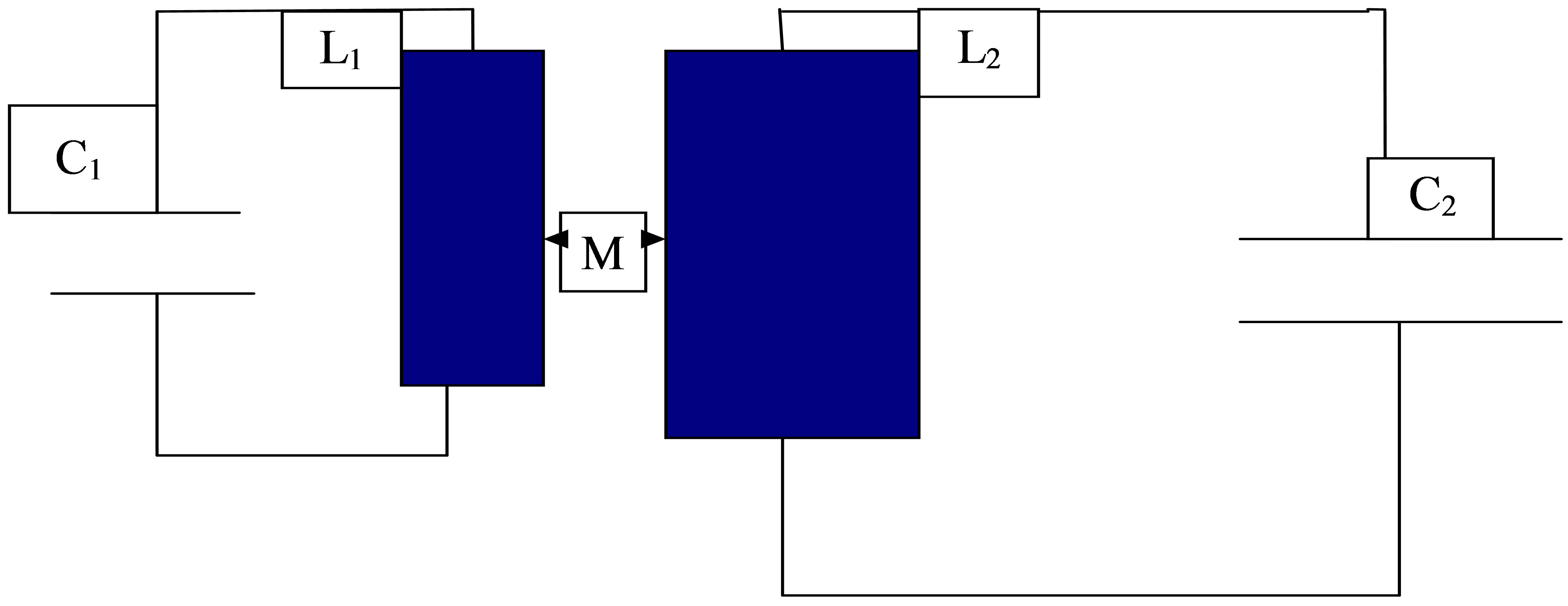
Figure 3. Magnetic coupling between 3 different oscillators.
|  (22) (22) |
|  (23) (23) |
Remarks: The substitution x = y + p/3 leads the equation x3 + ax + b = 0. The calculation procedure for a, b in terms of p, q, and r are given above in Equation (22). If one has calculated A, B in terms of a, b, then the 3 roots are readily computed. With respect to the 3 roots the following cases have to be regarded, where the solution of the matrix Equation (21) provides 3 normal modes (linear combination of cosine and sine):
 (24)
(24)
 (25)
(25)
It is again possible to construct “pendular movements” as previously carried out. The manifold increases considerably. We make use of the following definitions:
 (26)
(26)
The corresponding overall solution is as Equation (27).
By that we obtain 3 very slow difference frequencies (“pendular movements or beats”) and 6 fast (or very fast) frequencies. The 3 different beats may be connected with circadian, circasemi-septan and circaseptan, whereas the fast oscillations might have very short time periods (seconds, minutes or some hours).
2.5. Some Generalizations
The preceding section related to Figure 4 may be generalized by two extensions:
1) In addition to the magnetic couplings M12, M13, and M23 it is also possible to introduce connecting dielectric media between the capacitances. Then we have to extend all terms containing ω2, except the main diagonal elements, in Equation (21) by capacitive couplings. The calculation procedure of the eigenfrequencies is the same, only the parameters p, q, r, and consequently a, b, A, B in Equation (22) will contain further terms.
2) It is also possible to introduce a fourth oscillator; the coupling to other oscillators may be either magnetic and/or electric, and Equation (20) has to be extended to four different charges Q1,  , Q4:
, Q4:
 (28)
(28)
At every case, we have to solve a polynomial equation of fourth order, if we perform the substitution y = ω2:
 (29)
(29)
In a textbook [6] the procedure is described how to find the roots of this equation. A restrictive condition is that ω2 ≥ 0, but negative values have to be excluded. In terms of normal modes the general solution is given by:
 (30)
(30)
The manifold of “pendulum movements” of the charges between the oscillators is more interesting. On the other side, the difficulties to obtain suitable data also increase. The pendulum motions are given by Equation (31).
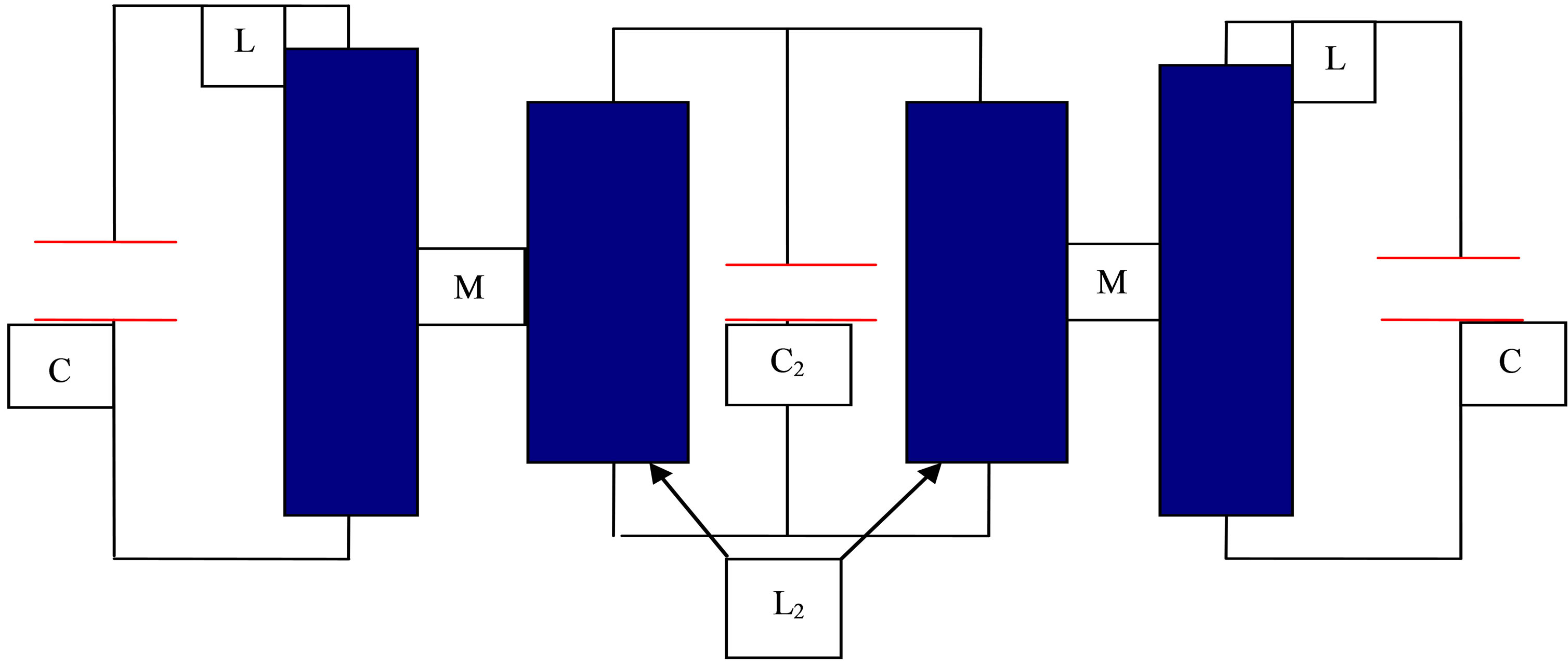
Figure 4. Coupled electric oscillators according to Equation (37).
| 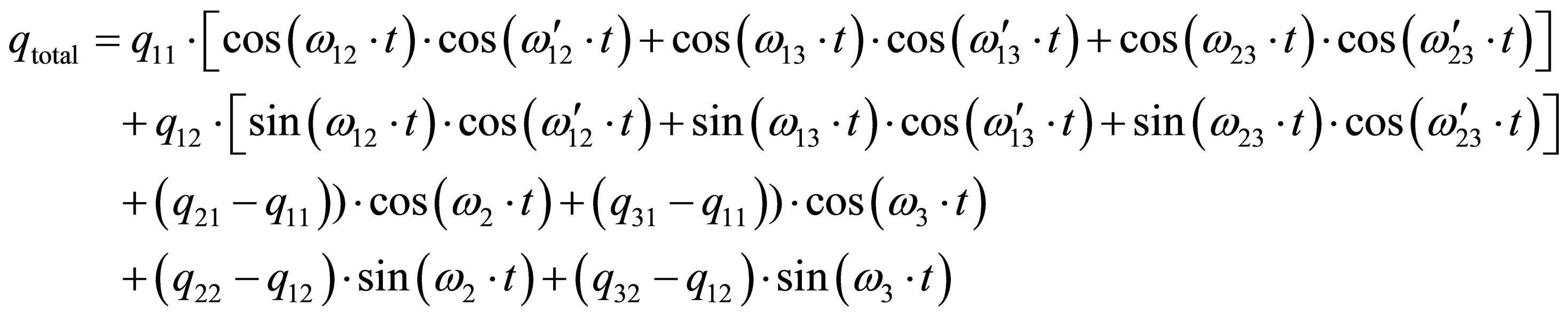 (27) (27) |
 (31)
(31)
Figures 5(a) and (b) are examples of such a generalization. We should mention that the mathematical treatment of 5 or more coupled oscillators implies numerical evaluations of the corresponding polynomial equations for the eigenfrequencies.
2.6. Aspects of Pendulum Movements (“Beat Frequencies”) of Coupled Circuits
In many fields of applied physics the signal analysis plays a dominant role. In particular, we remember its significance in information and/or control theory and the related technologies. In this case one considers, at least, two coupled electromagnetic circuits; the amplitudes of the normal modes satisfy q1 – q2 ≈ 0 (if more than two coupled circuits are applied, then q1 – q3 ≈ 0, q2 – q3 ≈ 0, etc should also be valid). This situation resembles a mechanical analogue, namely two pendulums with different masses and connected by a spring. In this case
 incorporates the extremely slow oscillating ground frequency and
  is a very fast modulation. The total energy needs a long duration to travel from one pendulum to the other one and to return. The pendular movement is therefore referred to as beat frequency (“beats”). The initial conditions have to be chooses such that the very slow ground frequency represents the carrier signal, i.e. q1 – q2 ≈ 0. In macroscopic systems it is always possible to satisfy such initial conditions.
With regard to molecular/cellular biology, where charge distributions of biomolecules (or even cells) are considered as capacitances and charge transfer processes (above all H bonds or interacting metallic ions) as currents, we do not know these initial conditions. This means that fast oscillations might be dominant, and only further components show “beats”, i.e. circadian, circasemi-septan and/or circaseptan periods. We have performed an analysis of beat frequencies, i.e. . It is very astonishing that even for cases where ω1 and ω2 refer to fast oscillations (T1 and T2 amount to ca. between 5 seconds and one minute), we are able to obtain numerous circadian, circasemi-septan and circaseptan periods. The only important property is that ω1 ≈ ω2 or T1 ≈ T2. Figures 6(a)-(d) show the yield of circadian, circasemiseptan, circaseptan and circatrigintan (ca. 30 days); examples have been studied by [7-10].
Figures 6(a)-(d) show the yield of circadian, circasemi-septan, circaseptan and circatrigintan period τ12 in dependence of T1 and T2. Those cases, where circadian or circasemi-septan, etc. are obtained, are significantly increased; therefore we do not show these connections. If we have, at this place, a look to transport phenomena and excitation processes in physics, then the following facts can be verified: transitions from singlet to triplet states may have life times in the order of seconds to minutes or longer.
If excited molecules are coupled or sites represent long molecular chains, then the excited state travels due to the proper coupling by inducing molecular deformations and intermediate changes of the electric charge. This is a more or less rather slow process; solitons behave in this
 (a)
(a) (b)
(b)
Figure 5. (a) Extension of the coupled circuits to a system with increased complexity compared to Figure 4; (b) Two different oscillators (L1, C1, L2, and C2) with electrical C12 coupling by an appropriate dielectric medium.
manner. Pure singlet excitations imply lifetimes of about 10−8 seconds. In molecular chains these excitations are referred to as excitons, which are damped by emission of light. Therefore the question arises, what are the principal processes leading to time periods with long durations (biorhythms) studied in chronobiology. Since τ12 may satisfy numerous different kinds of periods, if  is properly given, the chronobiological findings are not yet founded in satisfactory manner. In other words, we do not yet know the conductors for the preferences of some biorhythms leading to “beat time”. One way is to study correlations as performed by the Halberg group [7-10] and to analyze time series. However, we shall return to this question in the following sections.
2.7. Periodic Oscillators and the Transition to the Continuum
We continue Figure 2 by introducing further oscillators, where always the direct neighbors are coupled via M. Then we have to analyze the following system of equations :
:

 (32)
(32)
Equation (32) leads to the matrix Equation (33).
From matrix Equation (33) follows that the matrix has only diagonal elements of the form  and directs neighbors with the elements –Mω2/L. In the continuum
|  (33) (33) |
limit, this implies a wave equation. With regard to the magnetic coupling according to Equation (32), such a wave equation cannot be obtained. On the other side, periodic oscillators with magnetic coupling might have a restricted biological importance, since the periodicity is lacking in such systems.
It is interesting to note that for systems with periodic electric coupling we can derive a wave equation, similar to that considered in continuum physics obtained by periodic mechanical coupling. The analogue to Figure 3 is in the case of electric coupling:
 (34)
(34)
In the continuum limit, i.e. the distance Δx between the charges Qn+1, Qn and Qn−1 becomes infinitely small, Equation (34) assumes the shape:
 (35)
(35)
The term  represents the second derivative with regard to space, if lim Δx → 0 is carried out. Then we obtain a wave equation in the charge space:

 (36)
(36)
It should be mentioned that in the vacuum case the velocity v is equal to the velocity of light c. But v may be considerably smaller in the presence of a dielectric medium ε, i.e. v ≤ c. With regard to the presumption of Equations (32)-(36), namely a periodic system, the same comments are valid as previously pointed out: in biological systems the assumption of periodic boundary conditions may be rather idealistic in contrast to physics of crystals, where polarization waves of molecular crystals are studied. Therefore the study of some coupled oscillators may be more helpful. The inclusion of Ohm’s resistance R to be aware of damping (damped waves) is straightforward, and Equation (36) assumes the shape:
 (37)
(37)
The mechanical analogue of Equation (36) is a system of coupled oscillators with mass m and the force constant f. The equation of motion reads:
 (38)
(38)
By introducing the continuum limit in the fashion as in Equation (36) we obtain the wave equation of a string with regard to the amplitude (or elongation) q, i.e.
 (39)
(39)
In this case, v is the velocity of sound in the string. In contrast to electrical couplings, the string (solutions of Equation (39)) may satisfy well-known constraints, e.g. nodes (q = 0) at x = 0 and x = a. This constraint provides a discrete spectrum of modes:
 (40)
(40)
In Equation (40) λ refers to the wavelength and “a” to the distance of the string between the two nodes with q(0) = 0 and q(a) = 0. The continuum transition of coupled electromagnetic oscillators with M ≠ 0 according to Equations (32) and (33) can readily be carried out, but we obtain a “generalized” wave equation:
 (41)
(41)
In the continuum limit, we obtain from Equation (41):
 (42)
(42)
It is possible to express ω2 in terms of , which provides:
 (43)
(43)
Equation (42) is readily be solved by plane waves (Fourier expansion). Writing the k-vector in the form  we obtain:
 (44)
(44)
A consequence of the solution (44) is that, in spite of  might imply a fast oscillation of a single circuit, the coupling between the oscillators (chain with M ≠ 0) must lead to very slow oscillation frequencies
  and due to the following formula (45). This is in particular true for
 . The superposition of a ground wave with very slow periodicity and a faster modulation is also possible. This aspect might be interesting in chronobiology.
2.8. Standing Waves
The question arises, in which way standing wave solutions may become reasonable. For this purpose, we assume that the magnetic coupling M is interrupted at positions x = 0 and x = a. Then a proper wave mode excited within this interval cannot propagate into the domains x < 0 and x > a, and analogous boundary conditions hold as for the string. These boundary conditions can be satisfied for pure sine modes, i.e.
 (45)
(45)
Combining this result with Equation (44), we obtain:
 (46)
(46)
Due to the linearity of Equation (42) the superposition of the modes yields the following solution:
 (47)
(47)
The question arises, where in biology such a solution is applicable. Standing waves resulting from magnetic coupling are obtained, if at the “end-points” x = 0 and x = a, the coupling via M is interrupted by electrically neutral molecules. Then the excited wave amplitudes have to remain within this interval, and they form modes with the ground frequency (very slow) and faster modulations. Such a stationary state may breakdown, if at one endpoint a further molecule changes the nodal conditions and the coupling to the neighboring environment is established. The wave then escapes to reach a path or domain, which could not be reached before due to the lacking coupling interaction. This might be a possible mechanism and effect of neurotransmitters at a certain synapse. The escaped standing wave may be replaced by a new one, when the corresponding condition is reestablished and the wave is excited by further signals.
2.9. Theoretical Considerations of Resonance Interactions between Biomolecules and the Quantum Mechanical Base
The question arises in which way we can transfer quantum mechanical principles and results to problems of circuits, which represent charge distributions and currents influenced by magnetic fields.
2.9.1. Some Basic Aspects of phenomenological Correlations and Molecular Properties
It might appear that quantum theory cannot provide any information on the problem under consideration, namely resonances interacting molecules. According to a previous study [19] the interaction between molecules can describe the chemical affinity, which is phenomenological described by the Arrhenius equation, by the consideration of suitable term schemes and transition probabilities. This theory includes besides the specific affinity the transition to excited triplet states by visible light or by interaction between proper molecules, which can be characterized by their long life-time and superimposition of transport phenomena similar to diffusion processes. Moreover, the inclusion of magnetic fields and current is quite natural and based on a more fundamental theory as diffusion. The resonances can be viewed in light of circuits as previously considered. Although the previous study was mainly restricted to resonance interaction between drugs and DNA in order to explain very different correlations between cancerogenic molecules and mutagenicity, it can readily extended to other aspects such as quasi-degenerate triplet resonances of coupled oscillators, which are the main interest in this investigation. Therefore the question arises, what is connection between chemical affinity of biomolecules and their term schemes with biorhythms.
At first, we consider the classification of drugs with regard to the mutagenicity and, by that, to the carcinogenic effectivity. This problem has a long history, and the polycyclic aromatic hydrocarbons (PAHC) have been investigated by many authors with the help of quantum chemical means. Based on calculations of reactivity indices of ground state properties [11] the famous Kand L-region model has been developed to explain and predict the carcinogenic activity of some PAHCs. However, by inclusion of more available PAHCs than the Pullmans [11] had originally considered, numerous exceptions could be verified. Therefore this model did not contain the whole truth with regard to the connection between chemical structure/reactivity and carcinogenicity, and further quite different models have been proposed. We particularly mention the correlation of low excited states of PAHCs [12], charge transfer mechanisms (resonances) of PAHCs and DNA [13], and the connection between the dipole-dipole resonance interaction of PAHCs and excited states of the amino acid tryptophan [14], and the double resonance states of PAHCs with absorption of biophotons [15]. Since each of the mentioned correlations bears exceptions, a multiregression analysis has been performed to bring more light in this shortcoming of methodology [16], i.e. restriction to one molecular property.
According to [17-19] Figures 7(a)-(c) represent term schemes, which are characteristic for those molecules with a specific interaction with DNA or the amino acid tryptophan; the original restriction to PAHCs is superfluous. With the help of the transition probabilities of the related molecule sites the kind of interaction can be specified (chemical reaction, dipole-dipole resonance interaction, charge transfer, etc.). It should also be pointed out that the term schemes under consideration cannot be restricted to the original molecules, but the metabolites (produced by epoxydation, hydroxylation, carboxylation, etc.) usually show approximately the same term scheme with changed transition probabilities. Thus molecules characterized by the term scheme 7(c) the chemical reaction mechanism can be classified by biradicalic reactions [20].
 (a)
(a) (b)
(b) (c)
(c)
Figure 7. (a) Term scheme of double resonances of carcinogenic PAHCs. The solid arrow represents a permitted transition from the ground state to a higher excited state, whereas the dashes refer to a forbidden transition of the lower excited state to the ground state (the lifetime is significantly increased). The energy difference between these two excited states amounts to ca. 0.1 eV [15]; (b) This term scheme incorporates the same effect as Figure 7(a), the excitation of the excited triplet state from ground state is forbidden. Spin-orbit coupling permits radiationless transitions from the excited singlet state to the quasidegenerate triplet state. The lifetime of this state may be very long (order of seconds or minutes); (c) Term scheme of the cytostatic drug cyclophosphamide and metabolites [17,18]. The energy levels of the metabolites are only slightly changed, but the transition probability can drastically differ due to changes of spin-orbit coupling.
If for any mutagenic substrate or drug the base pairs of DNA or RNA incorporate the bioreceptors, one of the above term schemes should be applicable, and the ionization energy should also be comparable with the bioreceptor, i.e. ca. 6.9 eV - 7.7 eV. However, it is evident, that the presented findings may also be applied to other resonance interaction, e.g. with protein, hormones, etc. The term scheme may either be similar as it is the case for tryptophan and derivatives or rather different, if bioreceptors with other specific properties have to be accounted for. In every case, the chemical affinity between molecules according to the Arrhenius equations stands in close connection to resonance interactions derived by quantum mechanics. This is the subject of the next chapter.
2.9.2. Quantum Mechanical Aspects and Perturbation Theory
According to the methodology of quantum mechanics/ quantum chemistry there are two main approaches to describe the interaction between any two molecules A and B:
1) We assume the Hamiltonian H of the total system is of the form
 (48)
(48)
For the sake of simplicity, we suppose that the total system as well as the subsystems A and B shall remain in the singlet ground state. Then we have to calculate (e.g. Hartree-Fock, density functional, Feynman propagators or semi-empirical methods) the ground state energies of the subsystems A and B and of the total system in dependence on all nuclear co-ordinates (in realistic calculations restricted). The Hamiltonian H is assumed as usual (Coulomb interactions between electrons, nuclei, and between electrons among themselves). Magnetic interactions of charged particles, spin-spin and spin-orbit couplings are treated as perturbations and will be introduced separately. Although the total system shall remain in the singlet ground state, corrections by excited contributions via CI methods become then very essential, when A and B undergo interactions, since both molecules have to be stronger deformed and distorted. This fact is already true for separated molecules without the interaction term HAB, and the validity of the non-crossing rule is an indication for the relevance of excited configurations.
2) We assume that the Schrödinger equation for HA and HB is exactly/approximately solved:
 (49)
(49)
For the following considerations the impossibility of the first case is not relevant, since we can measure and classify the eigenstates and transition probabilities between the states under various conditions. Now we expand the eigenfunctions of H according to Equation (49) in terms of the eigenfunctions of HA and HB:
 (50)
(50)
We make use of the perturbation theory to classify the degree of the approximation (the applicability of the usual perturbation theory is assumed, since the states are not degenerate like isolated hydrogen atoms). The first order approximation is determined by the well-known relations for the coefficients (Equation (51)).
The second-order approximation does not provide any new principal insight, since only quadratic terms additionally appear (Equation (52)).
What are the implications of these results? We can verify that perturbation theory has many advantages in biochemical problems. The disadvantages of the approach (point 1) is easy to see: It is rather hopeless to compute the total systems “drug-bioreceptor” or “biomolecule-biomolecule”, and “bioreceptor” can be associated with a large biomolecule (DNA, RNA, protein, hormone). This approach is already hopeless, if one wishes to define the Hamiltonian of such a bioreceptor (one may think of the very complicated geometry of the double-stranded DNA including the H bonds between the base pairs interacting with chromatin). Therefore we have to restrict ourselves to theoretical means according to point 2, which also permit to use experimental properties (e.g. measurements of the ionization energy, excited states and transition probabilities inclusive intersystem crossings due to spin-orbit and spin-spin coupling). With respect to such a starting-point the methods of perturbation theory appear to be appropriate. We have already mentioned the correlation [14] (dipole-dipole interaction between tryptophan and any carcinogen) and the role of the excited states of the PAHCs in the domain 3.1 eV - 3.5 eV (Figures 7(a)-(c)). This may not be a contingency, since the lowest excited states of the nucleic acids also lie in this domain: guanine (G: 3.3 eV), adenine (A: 3.35 eV), thymine (T: 3.25 eV), cytosine (C: 3.45 eV) and uracil (U: 3.17 eV).
It is known that the triplet states are unaffected by the keto-enol tautomers, and in DNA or RNA we rather observe an energy band of triplet states within the above mentioned interval than separate energy levels (triplet conduction band [21]). The first excited singlet states are more influenced by the tautomeric equilibrium induced by the H bonds between certain base pairs. Therefore these excited states lie in the large domain between 3.7 eV and 4.7 eV. It should be mentioned that tryptophan possess two excited states between 4 eV and 4.3 eV, and the lowest triplet state is in the same interval as the triplet states of the nucleic acids. This property is also true for the derivates melatonin and serotonin, but the other amino acids (inclusive phenylalanine) only possess singlet and triplet states beyond 4.7 eV and 3.6 eV, respectively. At this position it should be pointed out that by accounting for the matrix elements of ground state and
|  (51) (51) |
|  (52) (52) |
excited states interactions and transition probabilities we are able to explain the chemical affinity between external molecule and bioreceptors such as DNA.
The Hamiltonian for a charged particle (e.g. electron, proton) in an external magnetic field and for spin-orbit/ spin-spin couplings has the form (details are given in [22-25]) (Equations (53a), (53b) and (54)).
 (53a)
(53a)
 (53b)
(53b)
The consequences of Equations (53a), (53b) and (54) are tremendous, since all magnetic interactions are accounted for, and the energy levels obtained by the Hamiltonians HA and HB are additionally splitted up. In contrast to usual applications, the mass  in Equation (53a) is related to a proton mass.
With Bz = B0 (Ax = −B0·y, Ay = Az = 0) the solution function of the Schrödinger Equation (53a) for free particles in a static magnetic field exhibits the form [22-24]:
 (55a)
(55a)
 (55b)
(55b)
 (55c)
(55c)
The function f(α) represents an arbitrary function; Hn refers to Hermite polynomials of the degree n with the energy eigenvalue En according to Equation (55b). Please note that for electromagnetic waves Equation (53a) is the basis for electric dipole transitions.
The expressions (I)-(III) have the following meanings: (I) refers to spin-orbit couplings of electrons in molecules, in cases to be explicitly mentioned (I) may also refer to protons. Expression (II) represents the spin-Pauli effect, i.e. the (small) interaction energy of the spin in an external magnetic field B0. With regard to additional electromagnetic waves (II) is responsible for transitions between different spin states induced by the waves. Expression (III) refers to spin-spin coupling (electron spinnuclear spin); it is usually very small and implies correspondingly small splitting of the energy levels. Since all contributions (I)-(III) described by Equation (54) certainly represent perturbations and splitting of discrete energy levels result from these properties, we state now the most important matrix elements (the Hamiltonian of spin-orbit coupling is denoted by HSO) (Equation (56).
If we look at the denominators of Equation (56) we again find the similar property as valid for the electronic interactions expressed by HAB, namely the energy difference has to be very small to record significant contributions of singlet-triplet transitions. The relevance of the term schemes 7(b) and (c) and their importance for the chemical reactivity are explained by these properties of the denominators. In contrast to the very fast pure singlet transitions the lifetime of triplet states has a particular meaning in long molecular chains, since charge and energy transport mechanisms are excited, which can lead to soliton transport in chains (e.g. muscles [26]) or activate H bonds.
The second contribution (II) may represent the interaction energy of the spin magnetic moment in an external magnetic field, i.e. a given energy level E is splitted up to yield:
 (57)
(57)
The magnetic moment  may either refer to the proton or electron moment,
  is the gyro-magnetic ratio. Contribution (II) also becomes relevant with regard to transitions between different spin states induced by electromagnetic waves; an example is NMR. The importance in the case of the much weaker geomagnetic field will be discussed later. The third contribution (III) refers to the coupling of spin with environmental spin systems and represents a transport mechanism with extremely low energy.
2.9.3. Consequences of the Resonance Denominators, Interactions with magnetic Fields and Couplings to Spin Systems to Problems of Chemical Affinity, H Bonds and Circuits
It is a general feature that all contributions (I)-(III) can be treated by well elaborated perturbation calculations, where in every order the energy differences appear in the denominators. The basic starting-point is incorporated by
|  (54) (54) |
|  (56) (56) |
the Hamiltonian H and its constituents HA, HB, HAB. Thus these constituents may belong to many-particle Schrö- dinger equations (they can be found in many textbooks of quantum mechanics, see e.g. [22-24], and/or nonlinear/ nonlocal Schrödinger equations with internal structure [2, 25]). The latter method also offers the possibility to calculate via charge densities and currents the properties of electric circuits in an easy manner. Furthermore, this approach incorporates in a quite natural way the density functional formalism, which has been put forward for the calculation of many-particle problems in biochemistry and molecular biology (e.g. the calculation of tunneling of protons between DNA base pairs [27-29]). Figures 8 and 9 incorporate the basis skeleton of the following calculations. The band structure (singlet and triplet states) of DNA is determined by the π electrons of the bases and the 3d-electrons of the phosphate ester [17-19]. These 3d-electrons exhibit a large coupling range of ca. 3.5 Å, which reaches besides neighboring π electrons of the same strand also 3d-electrons of the complementary strand, inclusive π electrons of the related nucleotides. A consequence of these properties is that the upper zone of

Figure 8. This figure includes the contents of the preceding Figures 7(a)-(c) (singlets: left, triplets: right); the presence of one (or more) further triplet states below the double resonance open new paths for interactions, e.g. propagation of triplet states.

Figure 9. Section of the double-stranded DNA helix and the H bonds (protons) between the base pairs A-T and G-C.
the triplet band (containing a huge number of discrete triplets) and the lower edge of the singlet excitation band overlap; a further essential property is the spin-orbit coupling of the 3d-electrons, which allows transitions from singlet to triplets and reverse. The arrows (solid lines) in Figure 8 are also valid in reverse direction, whereas the dashed arrows indicated processes with rather little probability. Owing to the splitting up of the triplet levels of 3d-electrons, we obtain an additional cascade of triplet states, which can serve as a pumping mechanism of energy, which may have its origin in ATP, GTP, etc.
It is a well-known property that the H bonds between the base pairs A-T and G-C modifies the local conformation of the DNA bases according to the position of the exchange protons (keto-enol tautomers). In particular, the excited singlet states are affected by the tautomerization, but with regard to triplet states the influence to band is less noteworthy [21]. A consequence of the difference in the local charge distribution of the ketoand enol tautomer is an asymmetric potential of the H bond, which is lowered in the keto conformation. Assuming a local temperature of 300˚K the proton tunneling velocity from the right-hand side (enol tautomer) of Figure 10 to the left-hand (keto tautomer) is fast, whereas for the reverse process the corresponding velocity is extremely small (factor 103). Since the charged tunneling protons incorporate spin 1/2 and a current between the corresponding base pairs, we can treat the energetic processes as perturbations. The influence of the geomagnetic field (order 0.5 × 10⁻⁵ Tesla) is rather difficult but very promising due to the helical structure of DNA:
1) If the direction of tunnel current between two base pairs is perpendicular to the direction of the geomagnetic field, then we have a maximum effect of the superimposed rotational motion induced by the Lorentz force (highest Larmor frequency).
2) If the direction of tunnel current between two base pairs is (approximately) parallel to the direction of the geomagnetic field, then we have a minimum effect of the superimposed screw induced by the Lorentz force (low-

Figure 10. Double minimum potential between the base pairs A-T. Left minimum: keto-tautomer of A (dashed line, model 2). Model 1 represents the symmetric approximation is valid for H bonds in water.
est Larmor frequency). Geomagnetic and solar magnetic fields have now about the same order of strength.
3) There are further configurations of H bonds between base pairs, where the projection of the magnetic induction B0 lies between the extreme cases 1 and 2.
The rotational motion of the protons induces additional spin-orbit couplings and spin-spin couplings with neighboring H bonds and 3d-electrons. The extremely small energy differences in the related dominators of the perturbation expansion of the wave functions yield sensitive resonances by external electromagnetic waves (with origins from the earth or the sun). The possible energy levels (singlets, triplets) of DNA suffer various further splitting, which can be excited by appropriate resonance conditions. In the language of electromagnetic circuits spinorbit and spin-spin couplings can be interpreted as mutual inductance M (cases (I) and (III) of Equation (54)). The interaction energy of the proton spin in the geomagnetic field is represented by the contribution (II) of this equation (spin-Pauli effect). The Lorentz force (interaction of the charged proton with the geomagnetic field) is expressed by the Hamiltonian (53a). This motion is quantized and leads to discrete energy levels expressed by the Larmor frequency (ground frequency). Excitations of the ground state can only occur by adsorption of electromagnetic waves with very low energy and proper eigenfrequency.
The asymmetry of the potential between DNA base pairs according to the dashed line of Figure 10 exhibits an additional interesting consequence. Due to the long probability of abidance in the keto conformation compared to the abidance in the enol conformation the helical DNA assumes an additional stability with regard to mutagenic influences. If a potential according to model 1 would be valid, then this property would not exist and the motion of a proton between the two minima due to quantum mechanical tunneling would be identical.
The additional circular motion of protons between base pairs seems to play also an important role in DNA replication and transcription, since it represents a key for the rotation specific parts of the DNA strands. Some consequences of calculations referring to this section will be discussed in Section 3.
Figure 10 results from a nonlinear/nonlocal field with internal structure and spin [2] (Equation (57)).
In lowest order, the solution functions can be approximated by the product wave functions
 (57a)
(57a)
Inclusion of higher order contributions of magnetic perturbations to the leading electrical part of the Hamiltonian  again implies resonance dominators as already pointed out for HAB.
The necessary integration procedure has already been worked out [2]; magnetic interactions by external fields and interactions with spin are treated as small perturbations. The realistic potential for tunneling protons between DNA base pairs is easy to handle by the generalized Gaussian convolution kernel K, which contains multipole expansions up to arbitrary order, accounted for in terms of two-point Hermite polynomials Hn.
3. Some Applications
In this section we consider problems of energy/charge transfer processes of DNA and the hydrolytic decomposition of ATP.
3.1. Properties of DNA
Figure 10 clearly shows that the H-bonds between DNA base pairs mediated by the protons represent a current. Since the current produced by each proton induces a magnetic field there exists a magnetic coupling. The strength of this coupling depends on phase properties, e.g. whether neighboring protons simultaneously run parallel or opposite between the base pairs. On the other side, the charge distributions in the DNA-basis coupled via deoxyribophosphates have to be regarded as coupled capacitances. The proton current between base pairs have been calculated with the help of Equation (57). This current is preferably affected by the geomagnetic field (Figures 11 and 12). Since the DNA exists as a double helix, it depends on the local orientation of the H bond related to the external field, whether Bgeomagnetic is fully or in a limit situation, very weak present due to the Lorentz force. Therefore the proton current cannot only occur along the smallest distance (straight-line) of the base pairs, but the corresponding motion represents an addi-
|  (57) (57) |

Figure 11. Directions of the geomagnetic field related to an H bond between the base pairs G and C. In Figure 11 f is extremely small (H bond and Bgeomagnetic are nearly parallel).

Figure 12. As Figure 11—the projection of Bgeomagnetic perpendicular to the axis between G and C is significantly higher.
tional screw. The rotational frequency is characterized by the Larmor frequency. In the limit case of a very small projection angle a further crew originated by the extremely small solar magnetic field may also influence the proton motion. Therefore the overall motion leads to further couplings along the H bonds of the double helix: spin-orbit coupling according to the rotational motion and spin-spin coupling between the moving protons and between protons and 3d-electrons of the phosphates of the nucleotides. Since the DNA bases of the strands mutually change configuration interactions (mixture of singlets and triplets with respect to keto-enol tautomers), the whole system of both strands represents resonators with dielectric coupling. With regard to the magnetic interactions along the double helix we have to account for rather weak couplings (spin-orbit and spin-spin). However, due to the H bonds mediated by tunnel currents between base pairs the wavelike motions (electric couplings between the bases of the related DNA strands and magnetic interactions) are not arbitrary; they coincide in the phases. The properties of Figures 11 and 12 in connection with Figure 10 are most important for biorhythms. Thus the potential according to Figure 10 is with slight modifications valid for all H bonds of DNA. If this potential would have the form of a flat minimum between the related base pairs, the protons would oscillate within this minimum according to the local temperature, any H bond would be possible between the base pairs and a keto-enol tautomerization would not exist. This means that the whole double-stranded helix could not exist in the real form. Since the interaction mediated by H bonds is connected with quantum mechanical tunneling, the frequencies of the protons travelling between base pairs are significantly lowered compared to thermal oscillations in a potential minimum.
At first, let us consider the H bond between A and T, G and C in connection with Figure 10. Thus the protons oscillate comparably fast within the corresponding potential minimum before successful tunneling can happen. This gives rise for an oscillating current expressed by inductivance L; the duration of halt probability at the bases is connected to the capacitance C. In first order, we can represent the 3 H bonds (G…C) by three identical oscillators (Figures 2 or 5(a), since they are not positioned in a coplanar way) and the two Hydrogen bonds (A…T) by Figures 2 or 3. Table 1 presents the results with/without magnetic couplings, which have been determined via calculations of the charges at the base pairs and currents between them.
The next step accounts for the magnetic interaction of protons of the H bonds in the geomagnetic field (Figures 11 and 12) leading to Larmor frequencies. Due to the double helix we can obtain all possibilities, i.e. a maximal effect, if proton motion and magnetic field are perpendicular, and a minimal influence, if both are parallel. In the latter case, the solar magnetic field can act with a very slow frequency. The time of resonances vary between 9 sec and 2 hours (if only the solar magnetic field is present under the particular configuration of the double helix). Since this motion exhibits always the form of circles around the axis between the base pairs, the geomagnetic field is permanently changing, which finally leads to mutual couplings between the protons travelling through and back and to spin-orbit/spin-spin couplings. A consequence of all these mutual couplings is that we obtain besides the fast oscillations “beat frequencies” of the order:
 (58)
(58)
In the continuum limit, which provides again standing

Table 1. Resonance frequencies of the H bonds of DNA with/without coupling between the corresponding base pairs A-T and G-C [27-29].
waves, we have also to account for these coupling. According to a previous section the related wave equation with asymmetric/nonlocal magnetic coupling reads:
 (59)
(59)
The asymmetric/nonlocal contributions result from weak couplings of longer/very long range. Therefore the coefficients a3 and a4 are given by the following Equation (60):
 (60)
(60)
Contributions of higher order can be neglected, but they indicate the complex situation of DNA. In similar fashion, the DNA bases along the strands are also connected in a nonlocal way, mainly due to the coupling via 3d electrons of the phosphate groups. Equation (36) now becomes:

 (61)
(61)
The standing wave solutions of Equations (45)-(47) cannot hold in Equations (59)-(61) due to the correction terms. Thus we obtain terms up to order 4, which now resemble the solutions of resonators consisting of 4 coupling terms. Due to spin-spin coupling we have also to add the existence of spin waves, of which the spin orientation is given by the direction of the geomagnetic field (so far other magnetic of stronger order are absent). If we replace in Equation (47) charge Q by spin S, an equivalent equation holds [22]. In a first order, Equation (62)
provides the already stated solutions:
 (62)
(62)
The difference to Equation (45) is only the weight factor c0, the eigenvalues are still unchanged:
 (63)
(63)
In further orders we account for the couplings. By that, we modify Equation (63) by adding the terms (note that c0 + c1 + c2 = 1).
The solution (64) is by no means complete. We should like to recall that M1·C and M2·C are related to resonance frequencies resulting from modifications of the basis frequency. The solution (64) provides “beat frequencies” with slow motions through and back along the DNA strands, i.e. the whole system is not rigid. These “beat frequencies” are related to the above values of τ0, τ1, τ2, τ3, but further numerical values in the intervals of relevance also exist.
The propagation of the changes of the configuration of the DNA bases obeys in the lowest order the solution (47), but we have also add correction terms (Equation (65)).
The solutions according to Equations (64) and (65) are not independent, since the values for ω, ω′, ω″ have to agree. In some model calculations, we have obtained the numerical values: c0 = 0.89, c1 = 0.09 c2 = 0.02, b0 = 0.87, b1 = 0.11 c2 = 0.02.
As already mentioned, this equation also exhibits standing waves. By specific interactions at some DNAsites and energy supply the double stranded DNA is opened in a wave-like fashion, e.g. via hydrogen bonds with water or a protein (see Figure 13).
|  (64) (64) |
|  (65) (65) |
3.2. Hydrolytic Decay of ATP-Mg-Protein Complexes
Figure 14 shows an ATP-Mg-protein complex, which one can find e.g. in the filaments of muscle cells. The energy of 0.5 eV is stored as a confined soliton [26]. The soliton can certainly be considered as a standing wave of a system of oscillators with electrical coupling. The presence of Ca2+ ions, water, tropomyosin, and troponin lead to the hydrolysis of ATP, and the coupling condition for standing waves, i.e. a node at the endpoints, breaks down. The stored energy escapes to become available for some other biomolecules, such as mechanical work of muscles, the muscle of the heart (very important) or synthesis of proteins, DNA replication and transcription, etc. It appears not to be probable that the stored soliton energy has very low frequencies. However, if Ca2+ ions show a 7- days-period due to the solar magnetic field, then it becomes evident that ATP hydrolysis also occurs with a 7- days-period [30,31]. The effect of the geomagnetic field leads to comparably fast oscillations (ca. 1 minute). The fast and slow oscillations occur simultaneously. Figure 14 presents the hydrolytic process in a schematic way. However, considering the magnetic interaction, this process is rather complicated. According to the results in Section 2.10.2 we have to account for the direction of the geomagnetic field and for the perpendicular component