LRS Bianchi Type-I Cosmological Model with Anisotropic Dark Energy and Special Form of Deceleration Parameter ()
1. Introduction
Our universe is undergoing a late-time accelerating expansion which has been evidenced by Riess et al. [1], Bahcall et al. [2], Bennett et al. [3], Spergel et al. [4], Cunha [5]. We live in a spatially flat universe composed of (approximately) 4% baryonic matter, 22% dark matter and 74% dark energy. Recently, Li et al. [6] studied the present acceleration of the universe by analyzing the sample of baryonic acoustic oscillation (BAO) with cosmic microwave background (CMB) radiation and concluded that such sample of BAO with CMB increases the present cosmic acceleration which has been further explained by plotting graphs for change of deceleration parameter q with redshift .
.
Many authors suggested a number of ideas to explain the current accelerating universe, such as scalar field model, exotic equation of state (EoS), modified gravity, and the inhomogeneous cosmology model. The dark energy EoS parameter is , where p is the darkenergy pressure and
  is its energy density. The value
  is necessary for comic acceleration. The simplest candidate for dark energy is the cosmological constant (
 ) for which
 . The matter with
  gives rise to Big Rip singularity (Caldwell [7]). Elizalde et al. [8] and Nojiri et al. [9] proposed several ideas to prevent the Big Rip singularity by introducing quantum effect terms in the action. Recently, Astashenok et al. [10] studied phantom cosmology without Big Rip singularity.
In the present paper, we have considered a LRS spatially homogeneous and anisotropic Bianchi type-I cosmological model with special form of deceleration parameter in general relativity. The physical and geometrical aspects of the model are also discussed. To have a general description of an anisotropic dark energy component, we consider a phenomenological parameterization of dark energy in terms of its equation of state  and skewness parameter
 . Some features of the evolution of the metric and the dynamics of the anisotropic dark energy fluid have been also examined. This paper is organized as follows. In Section 2, we have given the line element, energy momentum tensor and its parametrization and the field equations. In Section 3, isotropization and solutions are given. The physical and geometrical parameters such as the anisotropy parameter of expansion
 , the energy density
 , the deviation-free EoS parameter
  and the deviation parameter
  etc are also studied with proper interpretation.
2. Metric and Field Equations
The LRS Bianchi type-I line element is given by
 (2.1)
(2.1)
where  and
and  are the scale factors (metric potential) and functions of the cosmic time t only (nonstatic case).
Here we are dealing only with an anisotropic fluid whose energy-momentum tensor is in the following form
 .
.
We parametrize it as follows:
 (2.2)
(2.2)
where  is the energy density of the fluid,
  is the equation of state (EoS) parameters of the fluid and
  is the skewness parameter.
Here  and
and  are not necessarily constants and can be taken as functions of the cosmic time t.
The Einstein field equations, in natural limits ( and
and ) are
) are
 (2.3)
(2.3)
The Einstein’s field Equations (2.3) for metric (2.1) with the help of Equations (2.2) give
 (2.4)
(2.4)
 (2.5)
(2.5)
 (2.6)
(2.6)
where dot  indicates the derivative with respect to t.
3. Isotropization and the Solutions
We have three linearly independent Equations (2.4)-(2.6) with five unknowns  and
and . In order to solve this system completely, we use a special form of deceleration parameter as
 (3.1)
(3.1)
where  is mean scale factor of the universe and
  (>0) is constant.
This form has been proposed by Singha and(2.3)
The Einstein’s field Equations (2.3) for metric (2.1) with the help of Equations (2.2) giveal equation of state (EoS) parameter.
From Equation (3.1) after integrating, we obtain the Hubble parameter as
 (3.2)
(3.2)
where m is an arbitrary constant of integration.
Integrating twice Equation (3.1), we get  and the average scale factor as
 (3.3)
(3.3)
The spatial volume is given by
 (3.4)
(3.4)
i.e.
 (3.5)
(3.5)
here we consider .
.
The mean Hubble parameter  for LRS Bianchi type-I metric may be given by
 (3.6)
(3.6)
The directional Hubble parameters in the direction ,
,  and
and  respectively can be defined as
 (3.7)
(3.7)
Subtracting Equation (2.5) from Equation (2.6), we get
 (3.8)
(3.8)
Now, from Equations (3.4) and (3.8), we get
 (3.9)
(3.9)
Integrating, this gives
 (3.10)
 = constant of integration.
In order to solve above Equation (3.10), we use the condition
 (3.11)
Using Equation (3.11) in Equation (3.10), we obtain
 (3.12)
Now integrating Equation (3.12) and using Equation (3.5), we obtain the scale factors as
 (3.13)
 (3.14)
Using Equations (3.13) and (3.14) the directional Hubble parameters are found as
 (3.15)
 (3.16)
The mean Hubble parameter  for LRS Bianchi type-I metric may be given by
 (3.17)
The anisotropy parameter of the expansion is defined as
 where
where  represent the directional Hubble parameters in the directions of x, y and z axis respectively and is found as
 (3.18)
The shear scalar  , defined by
  is found as
 (3.19)
Using Equations (3.15), (3.16) and (2.4) we obtain the energy density as
 (3.20)
Using Equations (3.16) and (3.20) in Equation (2.5), we obtain the deviation-free parameter as

(3.21)
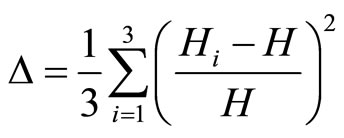
Now using Equation (3.11), we obtain the deviation parameter as
 (3.22)
The expansion scalar  is found to be
 (3.23)
4. Discussion
1) From Figure 1, one can verify that q decreases from  to
to  during evolution of the universe.
2) The dynamics of energy density  for LRS Bianchi type-I metric is illustrated in Figure 2. Here one can observe that all models [for different
 ] start with Big Bang having infinite density and as time increases (for finite time), the energy density tends to a finite value. Hence, after some finite time, the models approach to a steady state.
3) In Figure 3, we have plotted anisotropy parameter of expansion (D) against cosmic time t. For LRS Bianchi type-I model, it is observed that anisotropy parameter decreases to zero after some time. Hence, the model reaches to isotropy after some finite time which matches with the recent observations as the universe is isotropic at large scale.
4) The evolution of expansion scalar  for
for  is shown in Figure 4. It is observed that the expansion is infinite at
 . As cosmic time t increases, it decreases to a finite value
  after some finite value of t.
5. Conclusions
We have verified that the energy density of the fluid, the deviation-free equation of state parameter and the deviation parameter are all dynamical.

Figure 2. Energy density  vs cosmic time
 .
.

Figure 4. Expansion scalar  vs cosmic time
 .
.
It is observed that when , we get
 ,
,  and
and .
.
Which is mathematically equivalent to the cosmological constant (L CDM) model.
The SNe Ia data (Riess et al. [13], Astier et al. [14], Riess et al. [15]), the SDSS data (Eisenstein et al. [16]), and the three year WMAP data (Spergel et al. [17]) all indicate that the  model or the model that reduces to
  model is described as a standard excellent model in cosmology to describe the cosmological evolution. Hence, one can conclude that LRS Bianchi type-I cosmological model is the best fitted model as it reduces to
  model.
6. Acknowledgements
Authors are thankful to UGC, New Delhi for financial assistance through Major Research Project.