Mathematical Wave Functions and 3D Finite Element Modelling of the Electron and Positron

Declan Traill

Melbourne, Australia.

DOI: 10.4236/jamp.2024.124071                

Abstract

The wave/particle duality of particles in Physics is well known. Particles have properties that uniquely characterize them from one another, such as mass, charge and spin. Charged particles have associated Electric and Magnetic fields. Also, every moving particle has a De Broglie wavelength determined by its mass and velocity. This paper shows that all of these properties of a particle can be derived from a single wave function equation for that particle. Wave functions for the Electron and the Positron are presented and principles are provided that can be used to calculate the wave functions of all the fundamental particles in Physics. Fundamental particles such as electrons and positrons are considered to be point particles in the Standard Model of Physics and are not considered to have a structure. This paper demonstrates that they do indeed have structure and that this structure extends into the space around the particle’s center (in fact, they have infinite extent), but with rapidly diminishing energy density with the distance from that center. The particles are formed from Electromagnetic standing waves, which are stable solutions to the Schrödinger and Classical wave equations. This stable structure therefore accounts for both the wave and particle nature of these particles. In fact, all of their properties such as mass, spin and electric charge, can be accounted for from this structure. These particle properties appear to originate from a single point at the center of the wave function structure, in the same sort of way that the Shell theorem of gravity causes the gravity of a body to appear to all originate from a central point. This paper represents the first two fully characterized fundamental particles, with a complete description of their structure and properties, built up from the underlying Electromagnetic waves that comprise these and all fundamental particles.

Keywords

Electron, Positron, Wave, Function, Solution, Electromagnetic, Spin, Mass, Charge, Proof, Fundamental, Particle, Properties, Quantum, Mechanics, Classical, Physics, Computer, 3D, Model, Schrödinger, Equation, RMS, Klein, Gordon, Electric, Magnetic, Lorentz, Invariant, Hertzian, Vector, Point, Potential, Field, Density, Phase, Flow, Attraction, Repulsion, Shell, Theorem, Ehrenfest, Virial, Normalization, Harmonic, Oscillator

1. Introduction

In order to provide the foundations of a link between Classical Physics field concepts and the wave/particle duality in Quantum Mechanics, it is necessary to demonstrate how particles can be modeled both from a Classical Wave perspective while also satisfying the requirements of Quantum Mechanics, in particular the Schrödinger wave equation and the De Broglie equations. See Ref. [1] for the earlier work preceding this paper.

There is already evidence of this connection in the energy sum of the Electric and Magnetic fields in the Hamiltonian function that expresses the total energy of an atomic system:

Ref. [2] : “In 1926, Schrödinger used energy conservation to obtain a quantum mechanical equation in a variable called the wave function that accurately described single-electron states such as the hydrogen atom. The wave function depended on a Hamiltonian function and the total energy of an atomic system, and was compatible with Hertz’s potential formulation. The wave function depends on the sum of the squares of E- and H-fields as is seen by examining the energy density function of the electromagnetic field”.

In order to satisfy both the wave and particle natures of particles in a model of a particle, the particle’s wave function must satisfy both the Classical wave equation (which ensures that the wave function can represent a vibration of the space-time continuum) and the Schrödinger wave equation (which ensures that the wave function can represent a quantum of energy—thus a particle) [3] .

A wave function solution to the Classical wave equation describes the motion of all points on the wave at any location in space and time. The position of a test point in space as it is affected by the wave motion can be represented as a displacement vector drawn from the starting location of the point to its current location. The wave function defines the magnitude and direction of the displacement vector at any location in space and at any time—therefore, it completely and precisely defines the pattern of vectors that form the structure of the particle that it describes.

In the case of Electromagnetism, there is a single vector field that describes the motion of an Electromagnetic wave in this way, it is known as the Hertzian vector field [4] [5] . The Electric and Magnetic fields can both be derived from the Hertzian vector field by differentiation with respect to space and time.

Ref. [4] : “In a vacuum, a single Hertz vector written as the product of a scalar potential and a constant vector naturally arises as consequence of the transversality of the electromagnetic fields”.

Therefore, a wave function that describes a field of vectors representing Hertzian vectors can also represent a wave function describing Electric and Magnetic field vectors. If the wave function satisfies both the Classical wave equation and the Schrödinger wave equation, then it can also represent a vibration of space-time and a potential solution for a Quantum particle.

In the case of a Classical wave function describing an Electromagnetic wave, the displacement vectors described by the wave function are of a physical charge displacement from the otherwise neutral vacuum state. Thus, the vacuum is seen to be polarised by the displacement by an amount with units of Volt-Meters. The presence of the displacement from the neutral vacuum state requires a certain energy, and the total (rest) energy of the particle’s wave function is the sum of the resulting Electric and Magnetic fields [6] .

This paper presents two such solutions, one representing an electron and one representing a positron. In addition, it is shown that the correct Classical fields are produced by them, matching those of the real particles, and that the Quantum Mechanical requirements of the De Broglie equations are also met by them.

The form of these wave function solutions can be applied to ALL fundamental Physics particles, at all energy levels, and I have done the modelling and presented the wave function equations for a number of these particles already [7] [8] [9] .

1.1. History of the Development of the Wave Function Solutions

The wave functions I have determined are themselves initially complicated to look at—but they can be broken down into something quite simple. The wave function is of the form Aexp(a), where “A” is an Amplitude term and “a” is an angle term (exp is Euler’s exponential function). The wave function describes a field of vectors that rotate. The rate of rotation and the phase of each vector’s rotation are determined by the “a” angle term. This angle depends on both the distance “r” from the particle’s center, and on the time “t”. Don’t worry about the complex “i” term as it just means that the vectors are rotating in the complex plane—this is just to match the Schrödinger wave equations’ complex nature. In fact, both the wave equation and the wave function can be rewritten without any complex “i” but it takes a pair of equations rather than a single equation—and people are used to seeing the Schrödinger equation in its usual complex form. So, having a wave function that describes and field of rotating (Hertzian) vectors IS the omnipresent field of magnetic loops that Maxwell was referring to in his work [10] . As these Hertzian vectors are always spinning around, the d/dt of these vectors (Vector Potential A) always describes closed loops (Hence ߜA = 0) and Curl(A) describes the magnetic field B). Having determined the correct form of the wave function equation and proving that it was in fact a solution to both the Classical and Schrödinger wave equations, I had to determine what the correct values for “a” and “A” are. This was done by making the resulting wave function give the correct results for the De Broglie relations (for the “a” term) and the correct Electric Potential (V) (from the “A” term) and rest-mass energy (both the “a” and “A” terms).

As for what a wave function actually is, I had to teach myself this too, and also had some useful discussions on the old Wave Structure of Matter (WSM) Newsgroup whose aim was to describe the structure of matter in terms of waves (as the name suggests). One of the main proponents of the WSM newsgroup was Milo Wolff [11] who had proposed a spherically symmetrical model for the electron as a standing wave. This idea was a good first start, but had some problems, such as no apparent spin axis and the energy of the waves would blink into and out of existence many times per second—but one of the key principles of Physics that must be adhered to is that energy cannot be created nor destroyed—so there was an obvious problem with this model. My model solves both of these problems by introducing the spinning spiral structure that retains all the benefits of Milo’s model, yet provides a definite spin axis and a consistent energy content and also provides a mechanism by which electrostatic attraction/repulsion can occur [12] .

First of all, understand what a wave equation and wave function are. The Classical wave equation states a mathematical fact involving space and time parameters which is ALWAYS true for any traveling Classical wave. A wave function is an equation that is a solution to the wave equation—i.e. the wave function is the equation of the actual wave—which (if it is a solution to the wave equation) must be a valid Classical wave. What a wave function does is it connects space and time parameters in a way that can tell you the exact displacement position in space, of a hypothetical test point (such as a water molecule in a wave tank) at ANY moment in time. Thus, the wave function tells you everything there is to know about the wave—the exact positions of ALL points at EVERY possible time.

The Schrödinger equation is a specialized wave equation that imposes a slightly different mathematical relationship between the space and time parameters than the Classical wave equation. Essentially, it describes the conditions required for standing waves, or localized, discrete wave structures that persist over time without dissipating. Electron orbitals are one example of this, but in the case of electron orbitals, there is an additional term in the Schrödinger wave equation (in the Hamiltonian part) that states that the energy that is oscillating is in a (electric) potential field. This term is what causes the electron orbitals to have the shapes they do (rings, dumbbells, etc.) around the nucleus of an atom. I am using the Schrödinger equation to describe the electron cloud shape in the absence of an electric potential field—thus the cloud forms essentially a perfect sphere.

In the case of modelling the structure of fundamental particles purely from Electromagnetic waves (or Hertzian vectors to be precise—as all the other Electromagnetic properties can be derived from the Hertzian (Z) field) one needs to have a wave function that satisfies BOTH the Classical and the Schrödinger wave equations. The reason for this is that, as the particles are to be built from Electromagnetic waves, the Electromagnetic waves need to be Classical waves that form part of a continuum in space; and the wave function needs to also describe a localized, quantized structure—such that it describes a particle that doesn’t just dissipate into space instantly.

1.2. Lorentz Transformation of the Wave Function Solutions

The Schrödinger wave equation is not Lorentz Invariant, whereas the Klein-Gordon or Dirac equations (which are Lorentz Invariant) are usually used to model electrons/positrons. In my model, however, as the mass of the electron/positron does not appear as a point particle but is present as the mass equivalent of the total energy of in the Electromagnetic field (Electric and Magnetic fields combined) in the fields derived from the wave function equation [6] , the mass term in the Klein-Gordon and Dirac equations would be zero as the energy of the field is already accounted for in the other terms in these equations. The Klein-Gordon equation reduces to the Classical wave equation when the mass term is zero, and my wave function solutions are solutions to the Classical wave equation.

The Klein-Gordon equation [13] :

$\left[\square -{\left(\frac{mc}{\hslash }\right)}^2\right]\psi =0$

where: $\square ={\nabla }^2-\frac{1}{c^2}\frac{\partial }{\partial t^2}$ .

So, if m = 0:

${\nabla }^2-\frac{1}{c^2}\frac{\partial }{\partial t^2}\psi =0$

${\nabla }^2\psi =\frac{1}{c^2}\frac{\partial }{\partial t^2}\psi$

Which is the Classical wave equation.

The Classical wave equation is Lorentz Invariant, so my wave function solutions are also Lorentz Invariant. Therefore, my wave-function solutions are compatible with Relativity even though the Schrödinger wave equation (to which they are also solutions) is not a Relativistic wave equation. Another point to make here is that the wave functions are solutions to the Schrödinger wave equation (which applies in a frame that is at rest) and from Relativity we know that all inertial reference frames are equivalent—which means that Physics is the same for any moving observer. Therefore, we can conclude that the wave function in the moving reference frame is still a solution to the Schrödinger wave equation in that reference frame, even though that frame is moving with respect to us, and the Schrödinger wave equation itself is not Lorentz invariant.

2. The Solutions

These are the suggested wave function equations for the Electron and the Positron. Other work has suggested that the structure of the electron is that of a spherical standing wave [11] . That model has some problems, however, such as the resulting structure has no ability to explain the electron charge and would result in the waves all having zero amplitude at the same time during their oscillation cycle, which would cause problems with the conservation of energy. This model has been taken further and it has been found that in order to explain charge, the required structure is that of a spinning spiral wave, with inward or outward-flowing phase. These equations are formulated based on my initial analysis of the form of the structure that must be required—that of a spinning spiral with a spherical wave distribution. The equations were further refined with the use of the 3D modelling software developed by the author to simulate the wave functions. Also, the properties of these modelled wave functions were analysed to refine the amplitude term of the wave functions such that the electric potential of the modelled particles matches that of the real particles. Having done this gives good confidence that the resulting equations are a true description of the real fundamental particles.

The supplementary images at the end of this paper show graphical representations of the fields derived from these wave functions using a 3D vector modelling program developed by the author to aid in the visualization and testing of proposed wave function solutions.

For the Electron:

${\Psi }_e=\frac{Q_e\hslash }{4\pi r{M}_{e}c{\epsilon }_0}\exp \left[\frac{-i{M}_e{c}^2}{\hslash }\left(t-\frac{r}{c}\right)\right]$ (1)

For the Positron:

${\Psi }_p=\frac{Q_p\hslash }{4\pi r{M}_{p}c{\epsilon }_0}\exp \left[\frac{-i{M}_p{c}^2}{\hslash }\left(t+\frac{r}{c}\right)\right]$ (2)

where:

${\psi }_e$ = Electron wave function; ${\psi }_p$ = Positron wave function;

$Q_e$ = Electron charge (−); $Q_p$ = Positron charge (+);

$M_e$ = Mass of an electron; $M_p$ = Mass of a positron;

${\epsilon }_0$ = Permittivity of free space;

t = Time;

r = Distance from particle’s centre (to any location in space);

c = The speed of light;

$\hslash$ = The reduced Planck’s constant.

3. The Solutions Satisfy the Wave Equations

The wave nature of the particles is being modelled here as a vibration of the space-time continuum (a physical charge displacement) and the particle nature is modelled as localized quanta of this wave energy (a temporally stable 3D wave structure). In order to satisfy both the wave and particle natures of particles in the model, the wave function must satisfy both the Classical wave equation (which ensures that the wave function can represent a real, physical vibration of the space-time continuum) and the Schrödinger wave equation (which ensures that the wave function can represent a quantum of energy—thus a stable particle) [3] .

Classical wave equation: ${\nabla }^2\psi =\frac{1}{c^2}\frac{{\partial }^2\psi }{\partial t^2}$ (3)

Schrödinger wave equation: $i\hslash \frac{\partial \psi }{\partial t}=\hat{H}\psi$

where: $\hat{H}\psi =\text{Total}\text{Energy}$ ,

$\hat{H}\psi =\text{Kinetic}\text{Energy}\left(\text{KE}\right)+\text{Potential}\text{Energy}(\; PE\; )$

The wave function describes a field of rotating displacement vectors which can each be thought of as comprising two orthogonal Quantum Harmonic Oscillators [14] ; one along each axis of the complex plane. The vectors trace out a circle, such that at any given time half of the total energy is present as Kinetic energy (KE) and half as Potential energy (PE). The amount of energy in each these forms depends on the phase of each of the component Quantum Harmonic Oscillators. In their simple harmonic motion oscillation, each oscillates between full KE and full PE, but when one has full KE the other has full PE and vice-versa.

See Appendix A for the proof that a Quantum Mechanical wave function can be modelled as a field of real 3D vectors and still satisfy both the Schrödinger and Classical wave equations.

Due to Equipartition of energy in a Classical wave [15] :

$\text{KE}=\text{PE}=-\frac{{\hslash }^2}{2m}{\nabla }^2\psi$

So: $i\hslash \frac{\partial \psi }{\partial t}=-\frac{{\hslash }^2}{m}{\nabla }^2\psi$ (4)

Testing the electron solution with the Schrödinger wave equation

Referring to Equations (1) and (4):

In Spherical coordinates [16] , the Laplacian of ${\Psi }_e$ is:

${\nabla }^2{\Psi }_e=\frac{1}{r^2}\frac{\partial }{\partial r}\left(r^2\frac{\partial {\Psi }_e}{\partial r}\right)+\frac{1}{r^2\sin \theta }\frac{\partial }{\partial {\theta }^2}\left(\sin \theta \frac{\partial {\Psi }_e}{\partial \theta }\right)+\frac{1}{r^2{\sin }^2\theta }\frac{\partial {\Psi }_e}{\partial {\varphi }^2}$ (5a)

As the wave function ${\Psi }_e$ is symmetrical around its spin axis, all the vectors at the same distance r from the origin are identical, so the terms involving $\theta$ and $\varphi$ are zero.

So ${\nabla }^2{\Psi }_e$ reduces to:

${\nabla }^2{\Psi }_e=\frac{1}{r^2}\frac{\partial }{\partial r}\left(r^2\frac{\partial {\Psi }_e}{\partial r}\right)$ (6a)

Thus, the Schrödinger wave Equation (4) becomes:

$i\hslash \frac{\partial {\Psi }_e}{\partial t}=-\frac{{\hslash }^2}{m}\frac{1}{r^2}\frac{\partial }{\partial r}\left(r^2\frac{\partial {\Psi }_e}{\partial r}\right)$ (7a)

Thus:

$\frac{\partial {\Psi }_e}{\partial t}=\frac{i\hslash }{m}\frac{1}{r^2}\frac{\partial }{\partial r}\left(r^2\frac{\partial {\Psi }_e}{\partial r}\right)$ (8a)

As from ${\Psi }_e$ by differentiation of Equation (1), we can also say that:

$\frac{\partial {\Psi }_e}{\partial t}=\frac{-i{Q}_{e}c}{4\pi r{\epsilon }_0}\exp \left[\frac{-i{M}_e{c}^2}{\hslash }\left(t-\frac{r}{c}\right)\right]$ (9a)

Also:

$\frac{1}{r^2}\frac{\partial }{\partial r}\left(r^2\frac{\partial {\Psi }_e}{\partial r}\right)=\frac{-Q_e{M}_{e}c}{4\pi r{\epsilon }_0\hslash }\exp \left[\frac{-i{M}_e{c}^2}{\hslash }\left(t-\frac{r}{c}\right)\right]$ (10a)

Thus:

$\frac{i\hslash }{m}\frac{1}{r^2}\frac{\partial }{\partial r}\left(r^2\frac{\partial {\Psi }_e}{\partial r}\right)=\frac{-i{Q}_{e}c}{4\pi r{\epsilon }_0}\exp \left[\frac{-i{M}_e{c}^2}{\hslash }\left(t-\frac{r}{c}\right)\right]$ (11a)

So, from Equations ((8a), (9a) and (11a)), we can see that LHS = RHS of the Schrödinger wave equation (Equation (4)), so the wave function (Equation (1) is a solution to it:

$\frac{\partial {\Psi }_e}{\partial t}=\frac{i\hslash }{m}{\nabla }^2{\Psi }_e$

Equation (9a) equals Equation (11a):

$\frac{-i{Q}_{e}c}{4\pi r{\epsilon }_0}\exp \left[\frac{-i{M}_e{c}^2}{\hslash }\left(t-\frac{r}{c}\right)\right]=\frac{-i{Q}_{e}c}{4\pi r{\epsilon }_0}\exp \left[\frac{-i{M}_e{c}^2}{\hslash }\left(t-\frac{r}{c}\right)\right]$ (12a)

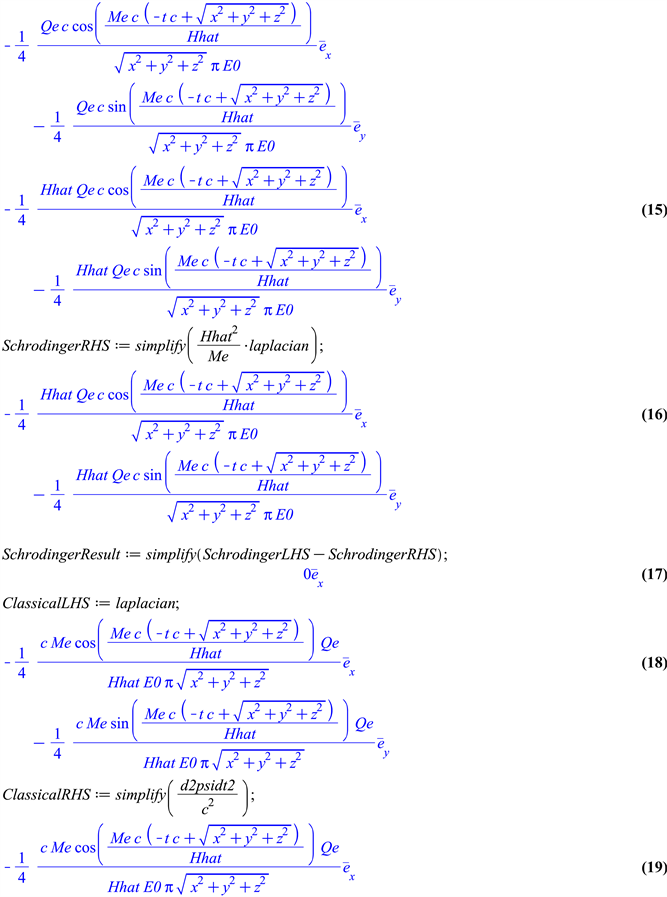
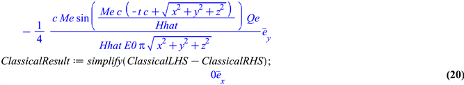
Testing the electron solution with the Classical wave equation

Referring to Equations (1) and (3):

$\frac{\partial {\Psi }_e}{\partial t}=\frac{-i{Q}_{e}c}{4\pi r{\epsilon }_0}\exp \left[\frac{-i{M}_e{c}^2}{\hslash }\left(t-\frac{r}{c}\right)\right]$ (13a)

So:

$\frac{{\partial }^2{\Psi }_e}{\partial t^2}=\frac{-Q_e{M}_e{c}^3}{4\pi r{\epsilon }_0\hslash }\exp \left[\frac{-i{M}_e{c}^2}{\hslash }\left(t-\frac{r}{c}\right)\right]$ (14a)

Thus:

$\frac{1}{c^2}\frac{{\partial }^2{\Psi }_e}{\partial t^2}=\frac{-Q_e{M}_{e}c}{4\pi r{\epsilon }_0\hslash }\exp \left[\frac{-i{M}_e{c}^2}{\hslash }\left(t-\frac{r}{c}\right)\right]$ (15a)

And, substituting Equations ((6a), (10a) and (15a)) into Equation (3):

$\frac{1}{r^2}\frac{\partial }{\partial r}\left(r^2\frac{\partial {\Psi }_e}{\partial r}\right)=\frac{-Q_e{M}_{e}c}{4\pi r{\epsilon }_0\hslash }\exp \left[\frac{-i{M}_e{c}^2}{\hslash }\left(t-\frac{r}{c}\right)\right]$

$\frac{-Q_e{M}_{e}c}{4\pi r{\epsilon }_0\hslash }\exp \left[\frac{-i{M}_e{c}^2}{\hslash }\left(t-\frac{r}{c}\right)\right]=\frac{-Q_e{M}_{e}c}{4\pi r{\epsilon }_0\hslash }\exp \left[\frac{-i{M}_e{c}^2}{\hslash }\left(t-\frac{r}{c}\right)\right]$ (16a)

So, LHS = RHS of the Classical Wave equation (Equation (3)) too, so the electron wave function (Equation (1)) is a solution to it also.

Testing the positron solution with the Schrödinger wave equation

Referring to Equations (1) and (4):

In Spherical coordinates, the Laplacian of ${\Psi }_e$ is:

${\nabla }^2{\Psi }_p=\frac{1}{r^2}\frac{\partial }{\partial r}\left(r^2\frac{\partial {\Psi }_p}{\partial r}\right)+\frac{1}{r^2\sin \theta }\frac{\partial }{\partial {\theta }^2}\left(\sin \theta \frac{\partial {\Psi }_p}{\partial \theta }\right)+\frac{1}{r^2{\sin }^2\theta }\frac{\partial {\Psi }_p}{\partial {\varphi }^2}$ (5b)

As the wave function ${\Psi }_p$ is symmetrical around its spin axis, all the vectors at the same distance r from the origin are identical, so the terms involving $\theta$ and $\varphi$ are zero.

So ${\nabla }^2{\Psi }_p$ reduces to:

${\nabla }^2{\Psi }_p=\frac{1}{r^2}\frac{\partial }{\partial r}\left(r^2\frac{\partial {\Psi }_p}{\partial r}\right)$ (6b)

Thus, the Schrödinger wave Equation (4) becomes:

$i\hslash \frac{\partial {\Psi }_p}{\partial t}=-\frac{{\hslash }^2}{m}\frac{1}{r^2}\frac{\partial }{\partial r}\left(r^2\frac{\partial {\Psi }_p}{\partial r}\right)$ (7b)

Thus:

$\frac{\partial {\Psi }_p}{\partial t}=\frac{i\hslash }{m}\frac{1}{r^2}\frac{\partial }{\partial r}\left(r^2\frac{\partial {\Psi }_p}{\partial r}\right)$ (8b)

As from ${\Psi }_p$ by differentiation of Equation (2), we can also say that:

$\frac{\partial {\Psi }_p}{\partial t}=\frac{i{Q}_{p}c}{4\pi r{\epsilon }_0}\exp \left[\frac{-i{M}_p{c}^2}{\hslash }\left(t+\frac{r}{c}\right)\right]$ (9b)

Also:

$\frac{1}{r^2}\frac{\partial }{\partial r}\left(r^2\frac{\partial {\Psi }_p}{\partial r}\right)=\frac{-Q_p{M}_{p}c}{4\pi r{\epsilon }_0\hslash }\exp \left[\frac{-i{M}_p{c}^2}{\hslash }\left(t+\frac{r}{c}\right)\right]$ (10b)

Thus:

$\frac{i\hslash }{m}\frac{1}{r^2}\frac{\partial }{\partial r}\left(r^2\frac{\partial {\Psi }_p}{\partial r}\right)=\frac{-i{Q}_{p}c}{4\pi r{\epsilon }_0}\exp \left[\frac{-i{M}_p{c}^2}{\hslash }\left(t+\frac{r}{c}\right)\right]$ (11b)

So, from Equations ((8b), (9b) and (11b)), we can see that LHS = RHS of the Schrödinger wave equation (Equation (4)), so the wave function (Equation (2)) is a solution to it:

$\frac{\partial {\Psi }_p}{\partial t}=\frac{i\hslash }{m}{\nabla }^2{\Psi }_p$

Equation (9b) equals Equation (11b):

$\frac{-i{Q}_{p}c}{4\pi r{\epsilon }_0}\exp \left[\frac{-i{M}_p{c}^2}{\hslash }\left(t+\frac{r}{c}\right)\right]=\frac{-i{Q}_{p}c}{4\pi r{\epsilon }_0}\exp \left[\frac{-i{M}_p{c}^2}{\hslash }\left(t+\frac{r}{c}\right)\right]$ (12b)

Testing the positron solution with the Classical wave equation

Referring to Equations (2) and (3):

$\frac{\partial {\Psi }_p}{\partial t}=\frac{-i{Q}_{p}c}{4\pi r{\epsilon }_0}\exp \left[\frac{-i{M}_p{c}^2}{\hslash }\left(t+\frac{r}{c}\right)\right]$ (13b)

So:

$\frac{{\partial }^2{\Psi }_p}{\partial t^2}=\frac{-Q_p{M}_p{c}^3}{4\pi r{\epsilon }_0\hslash }\exp \left[\frac{-i{M}_p{c}^2}{\hslash }\left(t+\frac{r}{c}\right)\right]$ (14b)

Thus:

$\frac{1}{c^2}\frac{{\partial }^2{\Psi }_p}{\partial t^2}=\frac{-Q_p{M}_{p}c}{4\pi r{\epsilon }_0\hslash }\exp \left[\frac{-i{M}_p{c}^2}{\hslash }\left(t+\frac{r}{c}\right)\right]$ (15b)

And, substituting Equations ((6b), (10b) and (15b)) into Equation (3):

$\frac{1}{r^2}\frac{\partial }{\partial r}\left(r^2\frac{\partial {\Psi }_p}{\partial r}\right)=\frac{-Q_p{M}_{p}c}{4\pi r{\epsilon }_0\hslash }\exp \left[\frac{-i{M}_p{c}^2}{\hslash }\left(t+\frac{r}{c}\right)\right]$ (16b)

So, LHS = RHS of Classical Wave equation (Equation (3)) too, so the positron wave function (Equation (2)) is a solution to it also.

4. The Wave Function and Electromagnetism

Each of the measurable fields in Electromagnetic Theory [5] [17] [18] , and their connection back to the wave function, can be expressed quite simply by the following set of equations and illustrated in Figure 1.

$A=-\frac{1}{c^2}\frac{\partial \psi }{\partial t}$ (17)

$V=\nabla \cdot \psi$ (18)

$E=\nabla V-\frac{\partial A}{\partial t}$ (19)

$H=\frac{-{\displaystyle \int \left(\nabla \times E\right)\partial t}}{{\mu }_0}=\frac{{\displaystyle \int \left(\nabla \times \nabla V\right)\partial t}}{{\mu }_0}-\frac{\nabla \times A}{{\mu }_0}=-2\frac{\nabla \times A}{{\mu }_0}$ (from Equation (3)) (20)

$\rho =-{\epsilon }_0\nabla \cdot E$ (21)

Figure 1. The mathematical connections between the fields.

Note: Equation (20) is derived from Equation (3) as the Classical wave equation states that $\nabla V=\frac{\partial A}{\partial t}$ , so H is equivalently:

$-\frac{\nabla \times A}{{\mu }_0}-\frac{\nabla \times A}{{\mu }_0}=-2\frac{\nabla \times A}{{\mu }_0}$

where:

$\psi$ = Wave function;

V = Voltage (electric potential);

E = Electric field vector;

A = Vector potential;

H = Magnetic field vector;

$\rho$ = Charge density.

5. Analysis of the Wave Functions

Both wave functions represent a field of rotating charge displacement vectors. The pattern described by the phases of the field of rotating vectors is that of a spinning spiral wave. As the waves move at the speed of light, they appear to be smooth fields without structure (such as the Electric Potential for the Electron/Positron (Figure 2)) unless probed at very short periods of time. The phase wave phase flows either away from or towards the centre of the particle (supplementary Figures S1-S4). The Electron spins with the phase wave flowing outward and the Positron with the phase wave flowing inwards [17] .

The angular frequency in the wave function is derived from the following three known equation:

$E=h\nu$ (22)

$E=m{c}^2$ (23)

$h=2\pi \hslash$ (24)

Substituting Equation (23) and Equation (24) into Equation (22) and solving for $\nu$ , we have:

$\nu =\frac{m{c}^2}{2\pi \hslash }$ (25)

Then to convert to angular frequency:

$\omega =2\pi \nu$ (26)

Substituting Equation (25) into Equation (26) and using the electron mass M_e gives:

$\omega =\frac{M_e{c}^2}{\hslash }$ Radians per Second (27)

This describes the rate of rotation of each of the vectors in the vector field that describes the Electron/Positron wave function.

The centre of the Electron comprises a vector that rotates around a fixed position at the particle’s centre over time. As time progresses this vector propagates radially outwards, at the speed of light, away from the centre thus forming the phase wave spiral. Therefore, the phase of each vector depends not only on time, but also on distance from the centre of the wave function.

So, the phase of each rotating vector in space will depend on two things:

1) The vector rotation rate, determined by:

$\frac{m{c}^2}{\hslash }$ (28)

2) The propagation delay for a wave travelling radially outwards at the speed of light, given the vector rotation rate above:

$\frac{m{c}^2}{\hslash }\times \frac{r}{c}$ (29)

Thus, the total phase change (for an electron) at a distance r from the centre is the sum of these two factors:

$\frac{M_e{c}^2}{\hslash }\left(t-\frac{r}{c}\right)$ (30)

Every point on the wave function spiral comprises a vector that rotates around a fixed location in space as the phase waves pass through each point.

In a classical wave, each point in the medium supporting that wave (such as the water molecules in a water wave) moves in a circular motion as the wave passes. The frequency of this circular motion is the same as that of the wave. However, when two waves of equal frequency (but travelling in opposite directions) combine to form a standing wave, each point in the medium rotates at twice the angular frequency of each of the two component waves.

The spinning spiral of rotating vectors that the wave function describes can be modelled as a standing wave comprised from two interfering waves: a spherical IN wave and a spherical OUT wave. Thus, each point in the medium supporting this standing wave is rotating at twice the frequency of either the IN or OUT wave alone.

The spherical IN and OUT waves work together, by means of constructive and destructive interference due to a slight frequency difference between the IN and OUT waves, forming the spinning spiral structure of the particle. Each point in this spatial structure is being influenced by both IN and OUT waves (one wave from each side), a vector at that point spins around at a rate based on the frequency of the IN and OUT waves, with an amplitude of double each of the IN and OUT wave components. The frequency of the IN and OUT waves is the same except for a slight difference that modulates this fundamental frequency and thereby forms the spinning spiral pattern.

The frequency of the vector rotation for any point in the wave function is given by Equation (27). Thus, the angular wave frequency of each IN/OUT wave is given by:

ω Radians per Second (31)

From Equation (26) and Equation (31), the travelling wave fundamental frequency of an IN or OUT wave is:

$\nu =\frac{\omega }{2\pi }\text{Hertz}$ (32)

So, from Equation (27) and Equation (32), the Electron’s IN/OUT wave frequency is:

$\nu =1.235590204456\times {10}^{20}\text{Hertz}$ (33a)

And (for a propagation speed of c) the spatial frequency (wavenumber) is:

$f_{electron}=4.12148528585\times {10}^{11}$ (33b)

6. Verification Using the De Broglie Equations

The De Broglie wavenumber for a moving particle is $\frac{m\nu }{h}$ (34)

This is 13,747.79 for an Electron travelling at 10 m∙sec⁻¹ (35)

The Classical interpretation of the De Broglie wave is that of a beat frequency of the upstream and downstream components (with respect to the particle’s direction of motion) of the Electron’s IN/OUT wave, so:

$f_{up}=f_{electron}\times \frac{c}{c-v}$ (36)

$f_{down}=f_{electron}\times \frac{c}{c+v}$ (37)

Again, the speed of the Electron v = 10 m∙sec⁻¹.

Thus, from Equation (36) and Equation (37), the beat frequency wavenumber is:

$\frac{f_{up}-f_{down}}{2}=13747.79$ (38)

So, we can see that the De Broglie wavenumber matches the beat frequency wavenumber of the calculated Electron IN/OUT waves for an Electron travelling at 10 m∙sec⁻¹ (Equation (35) equals Equation (38)).

The Energy of the Electron can be checked too, using the De Broglie relation:

$E=\hslash \omega$ (39)

Using Equation (27):

$E=\hslash \frac{M_e{c}^2}{\hslash }=M_e{c}^2$ (40)

Which is the Energy/Mass relationship as it should be.

This can also be proved using the displacement amount of the Quantum Harmonic Oscillators [14] in the wave function vector field. The units of the vectors in the wave function are Volt-Meters, so they need to be converted to just Meters, then the energy of the Oscillators calculated (see Appendix B).

The electron rest mass has also been calculated from my 3D model by integrating the Electric and Magnetic field vector energies over a small volume (cube) of space with the electron wave function at the center of the volume. The resulting rest-mass value is 100.46% of the actual electron rest-mass [6] .

7. Derivation of the Classical Electric Potential for the Electron and Positron

For the Electron wave function, the Electric Potential (V) is $\text{div}\left({\psi }_e\right)$ , which in spherical coordinates is [16] :

$\text{div}\left({\Psi }_e\right)=\frac{1}{r^2}\frac{\partial }{\partial r}\left(r^2{\Psi }_e\right)+\frac{1}{r\sin \theta }\frac{\partial }{\partial \theta }\left({\Psi }_e\sin \theta \right)+\frac{1}{r\sin \theta }\frac{\partial {\Psi }_e}{\partial \varphi }$ (41a)

For the Positron wave function, the Electric Potential (V) is $\text{div}\left({\psi }_p\right)$ , which in spherical coordinates is [16] :

$\text{div}\left({\Psi }_p\right)=\frac{1}{r^2}\frac{\partial }{\partial r}\left(r^2{\Psi }_p\right)+\frac{1}{r\sin \theta }\frac{\partial }{\partial \theta }\left({\Psi }_p\sin \theta \right)+\frac{1}{r\sin \theta }\frac{\partial {\Psi }_p}{\partial \varphi }$ (41b)

When viewed close-up, the spinning spiral and charge layers that comprise the Electron/Positron are clearly visible. Due to the fast spinning of the spiral (and outward or inward phase flow), or at large distance scales where the undulations of the spinning charge layers are small by comparison, the fields appear to become smooth and be of a continuous nature (Figures S5-S10). So, for example, the Electric Potential for the Electron/Positron (Figure 2) in this case appears to be the RMS (Root-Mean-Squared) [19] of Equation (41a) or Equation (41b), which is equal to the classical equation:

$\frac{Q_e}{4\pi r{\epsilon }_0}$ or $\frac{Q_p}{4\pi r{\epsilon }_0}$ (42)

For the Proof that this is the case, see Appendix C.

Figure 2. The electric potential of the electron wave function after it has been smoothed out by taking the RMS of the wave function over the 3D space it resides in.

8. Comparison with Quantum Mechanics

8.1. The Quantum Mechanical Wave Function

In Classical Physics, the wave function Ψ describes a field of displacement vectors; that is the complex number of the wave function describes X-axis and Y-axis displacements from the origin on an Argand diagram. In Quantum Mechanics, however, the wave function Ψ_QM is a complex scalar value rather than a vector, although the complex number of its wave function is in the same mathematical form. However, the complex “i” term in the wave equation simply represents a 90-degree rotation (orthogonal vector quantities), and so the equation can be reformulated purely Classically, with no complex numbers by introducing a rotation matrix in place of the “i” term [20] .

In Quantum Mechanics, the square of the wave function gives the probability density of finding a particle at a point in space:

$\rho ={\Psi }_{QM}^2$ (43)

In order to get vector quantities in Quantum Mechanics, one must apply a vector operator to the probability, such as applying the position or momentum operators to the wave function.

The Classical wave function, on the other hand, remains a vector and its magnitude is equivalent to the Quantum Mechanical scalar wave function:

${\Psi }_{QM}=\left|\Psi \right|$ (44)

As my Classical wave function solutions, Equations ((1) & (2)), are comprised of an array of Quantum Harmonic Oscillators, the Ehrenfest [21] [22] theorems state that the QM Expectation values follow their Classical trajectories and have an equipartition of energy (between Kinetic and Potential forms), so my Classical wave function solutions will also apply in a Quantum Mechanical interpretation.

See Appendix A for the proof that a Quantum Mechanical wave function can be modelled as a field of Real 3D vectors (with a rotation matrix in place of the complex “i” term) and still satisfy both the Schrödinger and Classical wave equations.

So, given that my Classical wave function model is compatible with the Quantum Mechanical wave function, this work sheds new light on the wave/particle duality issue in Quantum Mechanics. The Classical wave functions presented here for the particles is fundamentally a wave structure, yet the energy of this wave structure remains localized (quantized) and its properties appear to be associated with a single point—at the center of the wave function structure. As this wave structure is not a point particle but is spread through space with varying degrees of energy density in different locations, we can see how the probability amplitude referred to in Quantum Mechanics may be associated with the energy density and other properties of the dynamic waves of the Classical wave function.

8.2. Normalization of the Wave Function

In Quantum Mechanics, it is important that a wave function be normalizable; that is the area under the curve of the wave function is finite, such that the square of the wave function can represent a probability density of finding the particle. The probability integrated over the whole wave function must be 1, so that the particle exists somewhere in space. An infinite probability doesn’t make physical sense, so in order that the wave function represents a real particle, it must be Normalizable.

As my wave function solutions (Equations (1) & (2)) contain a 1/r term, they would not, on face value, appear to be normalizable due to an infinity at r = 0. However, if in reality, a function is known to be finite, as is the case for an electron or positron, then it may be considered Normalizable [23] [24] . As my wave functions are comprised of Quantum Harmonic Oscillators with real displacements in space, at size scales less than that displacement distance, the nature of the function will no longer be 1/r, thus restricting its amplitude and preventing an infinite quantity [25] . For these wave functions, the order of magnitude of this displacement is ~3.86 × 10⁻¹³ meters (see Ref. [14] ) on the physical displacement for a Quantum Harmonic Oscillator; in this case, assuming all of the energy of an electron was a single Quantum Harmonic Oscillator at the particle’s center). Thus, there is a natural limit on the 1/r factor in the wave-function amplitude. Thus, these wave functions are compatible with Quantum Mechanics, and their probability density may be calculated via Equation (43), with the use of Equation (44).

9. Conclusions

The wave functions presented here describe particles with all the correct properties for an Electron and a Positron and satisfy the requirements of both the Classical and Quantum Mechanical interpretations.

The wave function represents a field of rotating charge displacement vectors with units of Volt-Meters. The spinning vectors form a phase wave that describes a spinning spiral. The resulting phase wave flows either away from or towards the centre of the particle. Interactions between the phase waves of two or more particles can be shown to be the cause of the Electrical and Magnetic attraction/repulsion between charged particles due to momentum exchanges between the wave structures [12] .

In general, the concepts used to build these two wave equations could be applied to all particles in Physics. The key principles are:

1) The frequency of the waves that comprise the three-dimensional wave structure of the particle is based on the particle’s mass (via the calculation shown above).

2) A particle charge is defined by either an outward or inward flowing phase wave. A neutral particle would have no net phase flow inward or outward, but may contain regions of either inward or outward flow, which cancel out in the region surrounding the particle.

3) The completed wave function must satisfy both the Classical and Schrödinger wave equations.

4) Particles such as Protons (or other particles containing Quarks) might contain several components to the overall wave function [6] [7] [8] [9] [26] , which work together to form a stable particle (i.e. together they satisfy the other three principles stated here).

Further work can now, in principle, be done to determine the wave functions and thus structures of all of the known fundamental particles. The author has provided access to the programming code of the model used in this analysis (Appendix D) to allow other researchers to investigate this modelling further. The author has made some inroads into this endeavour in other work that suggests the wave function equations of the Proton [7] , the Neutron [8] and the Electron Neutrino [9] .

Supplementary Material

Images from the Model

Figure S1. The electron wave function from the side (the spin axis is vertical).

Figure S2. The electron wave function viewed from the top (looking down the spin axis).

Figure S3. The electron wave function (vector arrows only) viewed from the top (looking down the spin axis).

Figure S4. The electric potential of the electron showing the double spiral of charge layers.

Figure S5. The electric potential of the electron with the small-scale wave function undulations smoothed out (the individual charge layers are not visible).

Figure S6. The electric field of the electron with the small-scale wave function undulations smoothed out.

Figure S7. The magnetic field of the electron viewed from the side (spin axis is vertical) with the small-scale wave function undulations smoothed out. The vectors into/out of the page are not shown in order to reveal the nice magnetic field lines.

Figure S8. The magnetic field of the electron viewed from the top (looking down the spin axis) with the small-scale wave function undulations smoothed out.

Figure S9. The vector potential field of the electron viewed from the side (the spin axis is vertical) with the small-scale wave function undulations smoothed out.

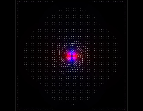
Figure S10. The vector potential field of the electron viewed from the top (looking down the spin axis) with the small-scale wave function undulations smoothed out. Note how the energy of the particle flows around the spin axis in closed loops.

Appendix A

Proof that a Quantum Mechanical wave-function can be modelled as a field of Real 3D vectors and still satisfy both the Schrödinger and Classical wave equations:

The Electron

See Ref. [20] for an example of the Schrödinger equation formulated without the use of complex numbers.

(The Positron calculation work out the same but use the different Ѱ function)

Appendix B

The wave function units are Volt-Meters, so by converting them to just Meters (by dividing by the Electric Potential (voltage) formula) and using the Energy of a Quantum Harmonic Oscillator field [8] , the energy of the Electron wave function can be shown to be the correct amount:

See Ref. [1] , Appendix C, page 63 for the full calculation.

Appendix C

Proof that the average (RMS) of the divergence of the wave function gives the Electric Potential field for the electron/positron, and that it is the same as the known Classical equation:

Here, the Wave Function is converted from Cartesian to Spherical coordinates and then the RMS is taken over both the $\theta$ angle coordinate when $\varphi$ is equal to π/2 (the equator of the wave function) to smooth the 3D spiral structure of the Wave Function into a continuous, smooth scalar field such as that of the Classical Electric Potential field. When this is done, the resulting field is compared to the Classical formula. There is a near perfect match between the two, with the only difference being factor based on $\hslash$ which has a value of 1.054571800E−34. This difference would be so small as to go un-noticed. There is, however, a larger proportion of the potential in the wave function along the equatorial plane, and a decrease (to nearly zero) along the polar axes in the spiral potential field of the original wave function (before the RMS is taken) which may be detectable in a well-constructed experiment.

The Electron

(The Positron calculation are the same but use the different Ѱ function)

See Ref. [1] , Appendix B, page 42 for the full calculations.

Appendix D

Field Calculation Code from the Model

See Ref. [1] , Appendix D, page 66 for the code listing. For the full modelling project’s code, see the GitHub project, Ref. [27] .

Conflicts of Interest

The author declares no conflicts of interest regarding the publication of this paper.

References

[1]	Traill, D. (2024) Wave Functions for the Electron and Positron 2013-2024. https://www.researchgate.net/publication/326646134_Wave_functions_for_the_electron_and_positron
[2]	(2015) A Brief Survey of the Various Field Equations since 1873. https://web.archive.org/web/20130408043138/ http://www.unifiedphysics.com/mathematics/
[3]	Simpson, G.D. (2015) Wave Equation and Rotation. http://vixra.org/abs/1208.0064
[4]	Ornigotti, A. and Aiello, A. (2014) The Hertz Vector Revisited: A Simple Physical Picture. Journal of Optics, 16, Article ID: 105705. http://iopscience.iop.org/2040-8986/16/10/105705 https://doi.org/10.1088/2040-8978/16/10/105705
[5]	Sein, J.J. (1989) Solutions to Time-Harmonic Maxwell Equations with a Hertz Vector. American Journal of Physics, 57, 834-839. https://doi.org/10.1119/1.15905
[6]	Traill, D. (2020) Electron Wave Function—Rest Energy Calculation. https://www.researchgate.net/publication/343206825_Electron_Wave_Function_-_Rest_Energy_Calculation
[7]	Traill, D. (2021) Proton Wave Function—Rest Energy Calculation. https://www.researchgate.net/publication/348691533_Proton_Wave_Function_-_Rest_Energy_Calculation
[8]	Traill, D. (2021) Neutron Wave Function—Rest Energy Calculation. https://www.researchgate.net/publication/348863139_Neutron_Wave_Function_-_Rest_Energy_Calculation
[9]	Traill, D. (2021) Neutrino Wave Function—Rest Energy Calculation. https://www.researchgate.net/publication/348691400_Neutrino_Wave_Function_-_Rest_Energy_Calculation
[10]	Maxwell, J.C. (1861) On Physical Lines of Force. Philosophical Magazine and Journal of Science. http://vacuum-physics.com/Maxwell/maxwell_oplf.pdf
[11]	Wolff, M. (2012) The Physical Origin of Electron Spin. http://mwolff.tripod.com/body_spin.html
[12]	Traill, D. (2020) Charged Particle Attraction and Repulsion Explained. A Detailed Mechanism Based on Particle Wave-Functions. https://www.researchgate.net/publication/342025994_Charged_particle_attraction_and_repulsion_explained_A_detailed_mechanism_based_on_particle_wave-functions
[13]	Oxford Reference (2021) Klein—Gordon Equation. https://www.oxfordreference.com/view/10.1093/oi/authority.20110803100039743
[14]	OpenStax (2020) The Quantum Harmonic Oscillator. Physics LibreTexts. https://phys.libretexts.org/Bookshelves/University_Physics/Book:_University_Physics_(OpenStax)/Book:_University_Physics_III_-_Optics_and_Modern_Physics_(OpenStax)/07:_Quantum_Mechanics/7.06:_The_Quantum_Harmonic_Oscillator
[15]	Duffin, R.J. (2015) The Equipartition of Energy in Wave Motion, 1969 Carnegie-Mellon University. http://repository.cmu.edu/cgi/viewcontent.cgi?article=1146&context=math
[16]	(2020) Gradient, Divergence, Curl, and Laplacian, LibreTexts. Del in Cylindrical and Spherical Coordinates. https://math.libretexts.org/Bookshelves/Calculus/Book:_Vector_Calculus_(Corral)/04:_Line_and_Surface_Integrals/4.06:_Gradient_Divergence_Curl_and_Laplacian
[17]	Traill, D. (2015) Towards a Unified Field Theory. http://gsjournal.net/Science-Journals/Research Papers-Mechanics / Electrodynamics/Download/1091
[18]	Kouzaev, G.A. (2010) Hertz Vectors and the Electromagnetic-Quantum Equations. Modern Physics Letters B, 24, 2117-2129. https://doi.org/10.1142/S0217984910024523
[19]	(2015) The RMS Voltage of an AC Waveform. http://www.electronics-tutorials.ws/accircuits/rms-voltage.html
[20]	Kadin, A.M. (2005) Quantum Mechanics without Complex Numbers: A Simple Model for the Electron Wavefunction Including Spin. https://arxiv.org/ftp/quant-ph/papers/0502/0502139.pdf
[21]	Krishnaswami, G.S. (2011) Notes for Quantum Mechanics 1 Course. https://www.cmi.ac.in/~govind/teaching/qm1-s11/qm1-lecture-notes-gk.pdf
[22]	LeBohec, S. (2015) Quantum Mechanical Approaches to the Virial. http://www.physics.utah.edu/~lebohec/ScaleRelativity/Virial/virial.pdf last accessed 11/6/2021
[23]	(2018) Wave Mechanics. https://ocw.mit.edu/courses/physics/8-05-quantum-physics-ii-fall-2013/lecture-notes/MIT8_05F13_Chap_01.pdf
[24]	(2018) Physics—Stack Exchange Discussion. https://physics.stackexchange.com/questions/107234/wave-function-not-normalizable
[25]	Gopalakrishnan, S. (2006) Self-Adjointness and the Renormalization of Singular Potentials. BA Thesis, Amherst College, Amherst, MA. https://web.archive.org/web/20170808113158/ https://www.amherst.edu/media/view/10264/original/gopalakrishnan06.pdf
[26]	Traill, D. (2021) Defining Quarks as IN/OUT Spherical Wave Components of the Proton’s Wave-Function. https://www.researchgate.net/publication/348870834_Defining_Quarks_as_INOUT_spherical_wave_components_of_the_Proton’s_wave-function
[27]	Traill, D. (2024) Vector Potential 3D Finite Element Modelling Software Project. https://github.com/Declan-Traill/VectorPotential