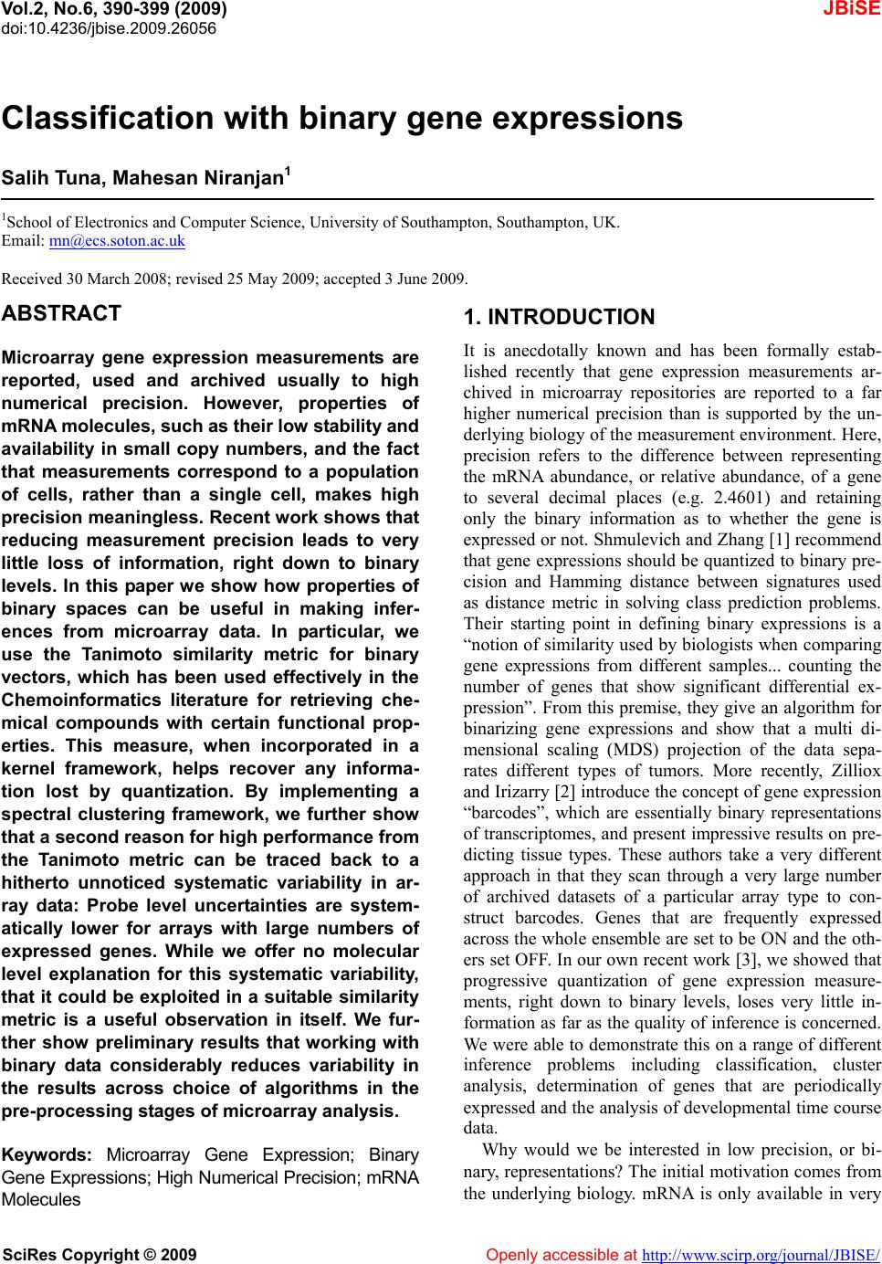
 Vol.2, No.6, 390-399 (2009) doi:10.4236/jbise.2009.26056 SciRes Copyright © 2009 Openly accessible at http://www.scirp.org/journal/JBISE/ JBiSE Classification with binary gene expressions Salih Tuna, Mahesan Niranjan1 1School of Electronics and Computer Science, University of Southampton, Southampton, UK. Email: mn@ecs.soton.ac.uk Received 30 March 2008; revised 25 May 2009; accepted 3 June 2009. ABSTRACT Microarray gene expression measurements are reported, used and archived usually to high numerical precision. However, properties of mRNA molecules, such as their low stability and availability in small copy numbers, and the fact that measurements correspond to a population of cells, rather than a single cell, makes high precision meaningless. Recent work shows that reducing measurement precision leads to very little loss of information, right down to binary levels. In this paper we show how properties of binary spaces can be useful in making infer- ences from microarray data. In particular, we use the Tanimoto similarity metric for binary vectors, which has been used effectively in the Chemoinformatics literature for retrieving che- mical compounds with certain functional prop- erties. This measure, when incorporated in a kernel framework, helps recover any informa- tion lost by quantization. By implementing a spectral clustering framework, we further show that a second reason for high performance from the Tanimoto metric can be traced back to a hitherto unnoticed systematic variability in ar- ray data: Probe level uncertainties are system- atically lower for arrays with large numbers of expressed genes. While we offer no molecular level explanation for this systematic variability, that it could be exploited in a suitable similarity metric is a useful observation in itself. We fur- ther show preliminary results that working with binary data considerably reduces variability in the results across choice of algorithms in the pre-processing stage s of microarray analysis. Keywords: Microarray Gene Expression; Binary Gene Expressions; High N umerica l Prec ision ; mRN A Molecules 1. INTRODUCTION It is anecdotally known and has been formally estab- lished recently that gene expression measurements ar- chived in microarray repositories are reported to a far higher numerical precision than is supported by the un- derlying biology of the measurement environment. Here, precision refers to the difference between representing the mRNA abundance, or relative abundance, of a gene to several decimal places (e.g. 2.4601) and retaining only the binary information as to whether the gene is expressed or not. Shmulevich and Zhang [1] recommend that gene expressions should be quantized to binary pre- cision and Hamming distance between signatures used as distance metric in solving class prediction problems. Their starting point in defining binary expressions is a “notion of similarity used by biologists when comparing gene expressions from different samples... counting the number of genes that show significant differential ex- pression”. From this premise, th ey give an algorithm for binarizing gene expressions and show that a multi di- mensional scaling (MDS) projection of the data sepa- rates different types of tumors. More recently, Zilliox and Irizarry [2] introduce the concept of gene expression “barcodes”, which are essentially binary representations of transcriptomes, and present impressive results on pre- dicting tissue types. These authors take a very different approach in that they scan through a very large number of archived datasets of a particular array type to con- struct barcodes. Genes that are frequently expressed across the whole ensemble are set to be ON and the oth- ers set OFF. In our own recent work [3], we show ed that progressive quantization of gene expression measure- ments, right down to binary levels, loses very little in- formation as far as the quality of inference is con cerned. We were able to demonstrate this on a range of different inference problems including classification, cluster analysis, determination of genes that are periodically expressed and the analysis of developmental time course data. Why would we be interested in low precision, or bi- nary, representations? The initial motivation comes from the underlying biology. mRNA is only available in very 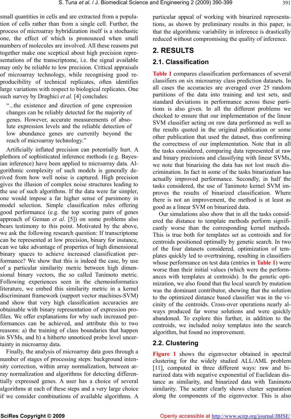 S. T una et al. / J. Biomedical Science and Engineering 2 (2009) 390- 399 SciRes Copyright © 2009 Openly accessible at http://www.scirp.org/journal/JBISE/ 391 small quantities in cells and are extracted fro m a popula- tion of cells rather than from a single cell. Further, the process of microarray hybridization itself is a stochastic one, the effect of which is pronounced when small numbers of molecules are involved. All these reasons put together make one sceptical about high precision repre- sentations of the transcriptome, i.e. the signal available may only be reliable to low precision. Critical appraisals of microarray technology, while recognising good re- producibility of technical replicates, often identifies large variations with respect to biological replicates. One such survey by Draghici et al. [4] concludes: “...the existence and direction of gene expression changes can be reliably detected for the majority of genes. However, accurate measurements of abso- lute expression levels and the reliable detection of low abundance genes are currently beyond the reach of microarray technology.” Artificially inflated precision can potentially hurt. A plethora of sophisticated inference methods (e.g. Bayes- ian inference) have been applied to microarray data. Al- gorithmic complexity of such models is generally de- rived from how well noise is captured. High precision gives the illusion of complex noise structures leading to the use of such algorithms. If the data were far simpler, one would impose a far higher sense of parsimony in model selection. Simple classification rules offering good performance (e.g. the top scoring pairs of genes approach of Geman et al. [5]) on some problems also bears testimony to this point. Motivated by the above, we ask the following research question: If transcriptome can be represented at low precision, binary for instance, can we take advantage of properties of high dimensional binary spaces to achieve increased classification per- formance? We show that this is indeed the case, by use of a particular similarity metric between high dimen- sional binary vectors, the so called Tanimoto metric. Following experiences seen in the chemoinformatics literature, we embed this similarity metric in a kernel discriminant framework (support vector machines-SVM) and show that very high classification accuracies are obtainable with binary representation of expression pro- files. We offer explanations for why such increased per- formances can be achieved, and attribute this to two reasons: a) the training of class boundaries that happen in SVMs, and b) a hitherto unnoticed probe level uncer- tainty in microarray data. Finally, the analysis of microarray data goes through a number of stages of processing steps: background inten- sity correction, within array normalization, between ar- ray normalization and algorithms for detecting differen- tially expressed genes. A user has a choice of several algorithms at each of these steps and a very large choice if we consider combinations of available algorithms. A particular appeal of working with binarized representa- tions, as shown by preliminary results in this paper, is that the algorithmic variability in inference is drastically reduced without compromising the quality o f inference. 2. RESULTS 2.1. Classification Table 1 compares classification performances of several classifiers on six microarray class prediction datasets. In all cases the accuracies are averaged over 25 random partitions of the data into training and test sets, and standard deviations in performance across these parti- tions is also given. In all the different problems we checked to ensure that our implementation of the linear SVM classifier acting on raw data performed as well as the results quoted in the original publication or some other publication that used the dataset, thus confirming the correctness of our implementation. Note that in all the tasks considered, comparing data represented at raw and binary precisions and classifying with linear SVMs, we note that binarising the data has not lost much dis- crimination. In fact in some of the tasks binarization has actually improved performance. Secondly, in half the tasks considered, the use of Tanimoto kernel SVM im- proves the results of binarized classification. Where there is not an improvement, the method is at least as good as a linear SVM on binarized data. Our simulations also show that in all the tasks consid- ered the distance to template methods perform signifi- cantly worse than the corresponding kernel methods. This is true both for templates set as centroids and for centroids positioned optimally by genetic search. In two of the four datasets considered, optimization of tem- plates quickly led to overtraining, resulting in classifiers whose performance on test data (entries in Table 1) were worse than their initial values (which were the perform- ances with templates at centroids). In the genetic opti- mization, we also found that the local search by mutation was the dominant contributor, showing that the solution to the optimized distance based classifier was in the vi- cinity of the centroids. Cross-over operations nearly al- ways produced far worse solutions and were quickly abandoned. To explore this further, in addition to the centroids, we included noisy templates into the search algorithm, but found no improvement. 2.2. Clustering Figure 1 shows the eigenvector obtained in spectral clustering for the widely studied ALL/AML problem [11], computed in three different ways: raw and bi- narized data with negative exponential of Euclidean dis- tance as similarity, and binarized data with Tanimoto similarity. The scatter clearly shows cluster separation along the components of the eigenvector. This is also 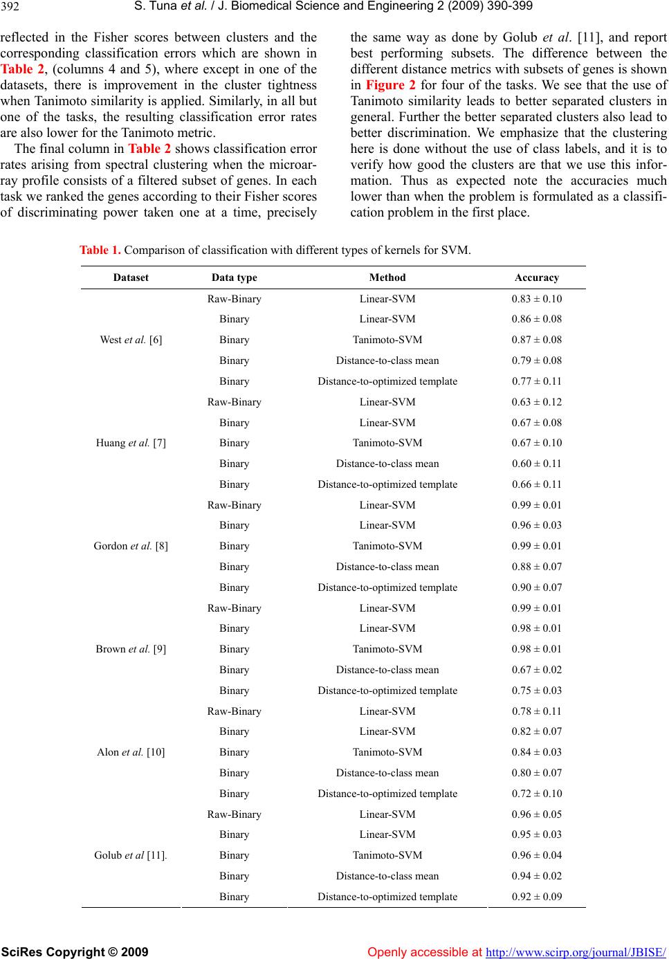 S. T una et al. / J. Biomedical Science and Engineering 2 (2009) 390- 399 SciRes Copyright © 2009 http://www.scirp.org/journal/JBISE/Openly accessible at 392 reflected in the Fisher scores between clusters and the corresponding classification errors which are shown in Ta b l e 2, (columns 4 and 5), where except in one of the datasets, there is improvement in the cluster tightness when Tanimoto similarity is app lied. Similarly, in all but one of the tasks, the resulting classification error rates are also lower for the Tanimoto metric. The final column in Table 2 shows classification error rates arising from spectral clustering when the microar- ray profile consists of a filtered subset of genes. In each task we ranked the genes according to their Fisher scores of discriminating power taken one at a time, precisely the same way as done by Golub et al. [11], and report best performing subsets. The difference between the different distance metrics with subsets of genes is shown in Figure 2 for four of the tasks. We see that the use of Tanimoto similarity leads to better separated clusters in general. Further the better separated clusters also lead to better discrimination. We emphasize that the clustering here is done without the use of class labels, and it is to verify how good the clusters are that we use this infor- mation. Thus as expected note the accuracies much lower than when the problem is formulated as a classifi- cation problem in the first place. Table 1. Comparison of classification with different types of kernels for SVM. Dataset Data type Method Accuracy Raw-Binary Linear- S VM 0.83 ± 0.10 Binary Linear- SVM 0.86 ± 0.08 Binary Tanimoto-SVM 0.87 ± 0.08 Binary Distance-to-class mean 0.79 ± 0.08 West et al. [6] Binary Distance-to-optimized template 0.77 ± 0.11 Raw-Binary Linear- S VM 0.63 ± 0.12 Binary Linear- SVM 0.67 ± 0.08 Binary Tanimoto-SVM 0.67 ± 0.10 Binary Distance-to-class mean 0.60 ± 0.11 Huang et al. [7] Binary Distance-to-optimized template 0.66 ± 0.11 Raw-Binary Linear- S VM 0.99 ± 0.01 Binary Linear- SVM 0.96 ± 0.03 Binary Tanimoto-SVM 0.99 ± 0.01 Binary Distance-to-class mean 0.88 ± 0.07 Gordon et al. [8] Binary Distance-to-optim ize d t emplate 0 .90 ± 0.07 Raw-Binary Linear- S VM 0.99 ± 0.01 Binary Linear- SVM 0.98 ± 0.01 Binary Tanimoto-SVM 0.98 ± 0.01 Binary Distance-to-class mean 0.67 ± 0.02 Brown et al. [9] Binary Distance-to-optim ize d t emplate 0 .75 ± 0.03 Raw-Binary Linear- SVM 0.78 ± 0.11 Binary Linear- SVM 0.82 ± 0.07 Binary Tanimoto-SVM 0.84 ± 0.03 Binary Distance-to-class mean 0.80 ± 0.07 Alon et al. [10] Binary Distance-to-optim ize d t emplate 0 .72 ± 0.10 Raw-Binary Linear- S VM 0.96 ± 0.05 Binary Linear- SVM 0.95 ± 0.03 Binary Tanimoto-SVM 0.96 ± 0.04 Binary Distance-to-class mean 0.94 ± 0.02 Golub et al [11]. Binary Distance-to-optim ize d t emplate 0 .92 ± 0.09  S. T una et al. / J. Biomedical Science and Engineering 2 (2009) 390- 399 SciRes Copyright © 2009 Openly accessible at http://www.scirp.org/journal/JBISE/ 393 (a) (b) (c) Figure 1. Figures showing spectral clustering results for different type of metr ics. In (a) spe ctral clustering is applied to continuous data by using Euclidean distance, in (b) binary data is used with Euclidean distance and in (c) binary data is used with Tanimoto coefficient for spectral clustering. Data from [11]. Table 2. Comparison of spectral clustering results by using Tanimoto and Euclidean distance with Fisher score and error rates. Dataset Data type Distance metrics Fisher score Error rate Error rate (best subset of genes) Raw Euclidean 2.47 ± 0.50 0.14 ± 0.08 Binary Euclidean 0.47 ± 0.49 0.33 ± 0.02 Simulated data Binary Tanimoto 0.66 ± 0.21 0.21 ± 0.10 Raw Euclidean 0.98 ± 0.41 0.32 ± 0.23 0.05 ± 0.11 Binary Euclidean 1.01 ± 0.43 0.10 ± 0.08 0.02 ± 0.04 Golub et al. [11] Binary Tanimoto 1.49 ± 0.42 0.05 ± 0.05 0.004 ± 0.02 Raw Euclidean 0.35 ± 0.22 0.21 ± 0.05 0.04 ± 0.05 Binary Euclidean 0.37 ± 0.18 0.22 ± 0.05 0.03 ± 0.05 Huang et al. [7] Binary Tanimoto 0.33 ± 0.17 0.21 ± 0.05 0.02 ± 0.04 Raw Euclidean 0.35 ± 0.04 0.45 ± 0.06 0.45 ± 0.06 Binary Euclidean 0.30 ± 0.18 0.33 ± 0.08 0.21 ± 0.15 West et al. [6] Binary Tanimoto 0.35 ± 0.24 0.28 ± 0.09 0.11 ± 0.07 Raw Euclidean 0.21 ± 0.07 0.17 ± 0.03 0.16 ± 0.03 Binary Euclidean 0.41 ± 0.19 0.13 ± 0.02 0.09 ± 0.03 Gordon et al. [8] Binary Tanimoto 0.52 ± 0.19 0.12 ± 0.02 0.08 ± 0.02  S. T una et al. / J. Biomedical Science and Engineering 2 (2009) 390- 399 SciRes Copyright © 2009 http://www.scirp.org/journal/JBISE/Openly accessible at 394 (a) (b) (c) ) (d) Figure 2. Comparison of spectral clustering results for four different datasets at various number of genes selected with Fisher Ratio. (a) is for [11], (b) is for [7], (c) is for [6] and (d) is for [8]. (a) (b) Figure 3. Reduction in variability of results due to preprocessing choice of algorithms. randomly chosen 38 combi- nations of preprocessing the CEL files produce large variations in classification results (leftmost columns). Working with discretized data reduces this variation in the inference. (a) data from [6], and (b) data from GSE2665. 2.3. Reduction in Algorithmic Variability Figure 3 shows reduction in the variability caused by choice of preprocessing algorithms. Patterns of gene expression levels change substantially with choice of algorithms, and this has a substantial effect on the re- sulting inference. A recent careful study (P. Boutros, personal communication1) established that this variabil- ity is significant. The leftmost columns of Figures 3(a) and (b) show this as box plots on two datasets. We see 1Also presented at the Microarray Gene Expression Society (MGED) meeting, Riva del Garda, Italy, September 2008.  S. T una et al. / J. Biomedical Science and Engineering 2 (2009) 390- 399 SciRes Copyright © 2009 Openly accessible at http://www.scirp.org/journal/JBISE/ 395 standard deviations in classifier performances, with out- liers removed, of 0.032 and 0.134 re spectively, and th ese reduce to 0.017 and 0.009 when th e ex pr essio n leve ls ar e binarized. The use of Tanimoto metric (box plots of the last columns of Figure 3) improves this even further. 3. DATA AND METHODS 3.1. Approach Our approach was to show that on a sample of classifi- cation problems published in literature, classification accuracies reported by the authors do not significantly degrade when the gene expression data is quantized to binary precision (i.e. if the gene is expressed or not). Having achieved this, we implemented a similarity measure suitable for high dimensional binary spaces in a kernel framework to show that any loss of performance is easily recovered. In a number of cases the approach we took indeed produced better accuracies than working with the data at raw precision (see Results). 3.2. Tanimoto Similarity Tanimoto coefficient ( ) [12], between two binary vec- tors, is defined as follow: cba c T where a: the number of expressed points for gene x, b: the number of expressed points in gene y and c: the number of common expressed points in two genes. Tanimoto similarity ranges from 0 (no points in com- mon) to 1 (exact match) [13] and is the rate of the num- ber of common bits on to the total number of bits on two vectors. It focuses on the number of common bits that are on. The denominator of Tanimoto coefficient can be considered as a normalization factor which helps to re- duce the bias of the vector size (i.e with larger vectors Tanimoto coefficients work better [14,15]. For this rea- son Tanimoto coefficient is the preferred similarity measure in chemoinformatics as all the vectors are long and there are only few bits on. Tanimoto kernel can be defined as [16]: zx zxK TTT T Tan ),( where , and . It follows from the work of Trotter [16] that this similarity metric satisfies Mercer conditions to be useful as a valid kernel: i.e. kernel computations in the space of the given binary vectors map onto inner products in a higher dimensional space so that SVM type optimizations for large margin class boundaries is possible. xxa T zzbT zxcT Alternate ways of classification of binarized data can be considered. Motivated by the distance to barcode classifier built by Zilliox and Irizarry [2] we imple- mented similar classifiers. An obvious choice in these circumstances is to set two templates, one to represent each class, and position them at the centroids of the two class profiles. This is a distance to mean classifier in standard statistical pattern recognition terminology. A particular limitation of this strategy is discussed later. The barcodes designed by Zilliox and Irizarry [2], how- ever, are not positioned at the centroids because they are evaluated by analysing a large number of archived ex- periments. We also built such discriminant templates, by doing a stochastic search starting from the centroids as initial condition. Such an optimization achieves tem- plates that are better positioned in the input space than centroids for distance-base d di scri mination. Clustering is the most popular tool in the analysis of microarray data. In order to conform whether the use of Tanimoto distance metric is useful in clustering, we ap- plied the method of spectral clustering to the classifica- tion problems considered above. Without knowledge of the class labels, we clustered each of the datasets into two clusters using spectral clustering. Subsequently, us- ing knowledge of the class labels we looked to see how well separated the clusters formed were, and how accu- rately the data was allocated to the right clusters. To measure cluster compactness we used the Fisher ratio as performance metric: Fisher Score = 21 21 )( abs Checking if the examples were consistently associated with the right clusters, we computed percentage classifi- cation errors. The choice of classification problems to evaluate cluster compactness offers a far better setting than clustering genes into functions. This is because cluster analysis, when the data has large numbers of clusters in them, is notoriou sly unstable. With data taken from classification problems, we could expect well de- fined cluster formations (e.g. cancer versus non-cancer), in which we can compare the role of different distance metrics. 3.3. Datasets We give a short description of the datasets used in our study. Yeast dataset compiled and first used in Brown et al. [9] for predicting yeast gene functions. cDNA arrays, in which the task is to classify 121 ribo- somal genes from the remaining 2346 using 79 features. The features are hybridization conditions during cell cycle progression under different syn- chronization methods. Widely used Leukemia dataset (Golub et al., [11]); there are 5000 genes with 38 samples (27  S. T una et al. / J. Biomedical Science and Engineering 2 (2009) 390- 399 SciRes Copyright © 2009 Openly accessible at http://www.scirp.org/journal/JBISE/ 396 ALL, 11 AML), being the test subset of the full dataset. Colon da taset (Alon et al., [10]), 2000 genes with 62 samples (20 normal and 42 tumour samples). Two Breast cancer datasets, first one from (West et al., [6]) 7129 genes and 49 samples, (25 ER+ and 24 ER-) and the other Huang et al. [7] 12625 genes with 89 samples (depending on LN status). Lung cancer dataset, (Gordon et al., [8]), 12533 genes and 181 samples (31 malignant pleural mesothelioma (MPM) and 150 adenocarcinoma (ADCA)). 53 randomly selected datasets from ArrayExpress (http://www.ebi.ac .uk/ar rayexpress/) and Gene Expression Omnibus (GEO) (http://www.ncbi.nlm.nih.gov/geo/) for probe level uncertainty analysis analysis. Accession numbers of these datasets are: GEO: GSE5666, GSE7041, GSE8000, GSE8505, GSE6487, GSE6850, GSE8238, GSE2665 Array Express: E-GEOD-6783, E-GEOD-6784}, E-MEXP-1403, E-ATMX-30, E-GEOD-6647, E-GEOD-6620 , E-ATMX-13, E-MEXP-1443, E-GEOD-2450, E-GEOD-2535 , E-MEXP-914, E-MEXP-268, E-GEOD-2848, E-GEOD-2847 , E-MEXP-430, E-GEOD-6321, E-MEXP-70, E-GEOD-1588, E-MEXP-727, E-TABM-291, E-GEOD-3076, E-GEOD-1938 , E-GEOD-7763, E-GEOD-3854 , E-GEOD-1639, E-TABM-169, E-MAXD-6, E-MEX P-526, E-GEOD-2343, E-GEOD-3846 , E-MEXP-26, E-GEOD-1723, E-GEOD-1934, E-MAXD-6, E-MEXP-879, E-GEOD-10262, E-GEOD-10422, E-MEXP-998, E-MEXP-580, E-GEOD-10072, E-GEOD-10627. Web Pages: http://yeast.swmed.edu/cg i-b in/dlo ad. cgi, http://data.genome.duke.edu/west.php, http://data.genome.duke.edu/lancet.php, http://chestsurg.org/publications/2002-microarray.aspx Synthetic data was produced following Dettling [17], using R code made available by the au- thors. Data is produced to follow the statistics (mean and correlation structure) of the leukae- mia data [11]. We generated several realizations of 200 samples in 250 dimensions. We explored varying these values over a range, and results reported in this paper correspond to the above figures. 3.4. Spectral Clustering Spectral clustering uses eigenvectors of the pairwise similarity matrix to partition the data. The most widely used distance metric to calculate the similarity matrix is the negative exponential of a scaled Euclidean distance. 2 2 ),( exp ji ji xx A where the scale parameter is a free tuning parameter. The steps involved in spectral clustering, in which we replace the similarity measure by Tanimoto similarity between binary strings, are summarized as follows: Pairwise similarity matrix ji A, between the genes i and j is calculated by us ing Tanimoto coef- ficient. Following Brewer [18] an exponential is applied: 2 )1( exp ij A F ij A Compute the normalized Laplacian matrix. 2/12/1 D DL F Compute the eigenvalue decomposition of L. iii DyyLD )( Select the eigenvector corresponding to the second smallest eigenvalue. Parameters and were tuned by searching over a range of feasible values: –5.05.0. Uncertainties in results for cluster analysis were evaluated by a bootstrap method. For each of the tasks, 100 datasets of the same size as the original data were created by sampling with replacement before the appli- cation of the spectral clustering algorithm. Perfor- mances reported are averages and standard deviations across these 100 bootstrap samples. 3.5. Optimised Templates The search to find templates better than class means for a distance-to-template classifier was implemented as a stochastic local search by means of a genetic algorithm. Templates were initialized to class means. At every step in an iterative search, we randomly changed 20% of the elements in the two templates, to derive mutated bar- codes in their vicinity. Throughout the search, we re- tained ten best template pairs at any iteration. Large search steps were implemented by crossover operation between pairs of templates whereby half the bits in the patterns were swapped between pairs, a standard opera- tion in genetic algorithms. We evaluated the accuracy of the resulting classifier and there was an improvement we retained the mutated templates, and discarded them if was no improvement.  S. T una et al. / J. Biomedical Science and Engineering 2 (2009) 390- 399 SciRes Copyright © 2009 http://www.scirp.org/journal/JBISE/ 397 that classification by computing distances to a template is optimal only in the case that the distributions of each class is Gaussian, isotropic (i.e. variances of each feature is the same) and these variance s are the same for both [22 ]. 3.6. Algorithmic V ariability We used the EXPRESSO set of algorithms in package Affy in Bioconductor. For both datasets West et al. [6] and GSE2665, we worked from the CEL files and app- lied a total of 38 different preprocessing combinations from a total of 315 possibilities, randomly chosen. When any of these assumptions is violated, a distance to template classifier is no longer optimal. Even under the mild relaxations of the assumption, that of Gaussian den- sities with identical but nonisotropic covariance matric- 3.7. Other Details es, the optimal classifier requires computation of second order statistics in the form of the Mahalanobis distance to class means. In gene expression data isotropic v ari a tio n cannot be assumed. Under regulation by combinatorial transcription factor activity where each transcription fac- To analyse probe level uncertainties (Milo et al. [19]) we used the PUMA package (Propagating Uncertainty in Microarray Analysis), downloaded from the site (www.bioinf.manch ester.ac.uk/resources/pu ma/). For quantization of microarray data, we used the method developed by Zhou et al. [20], which models gene ex- tor may control several genes, correlated expression of groups of genes should be expected. Indeed, the wide use of cluster analysis of microarray data is based on the assumption that correlated expression profiles might su- pressions as mixture Gaussian densities. For quantiza- tion to binary levels, two Gaussians are used, resulting in two means and standard deviations:1 ,2 ,1 and 2 . ggest co-regulation. Therefore, as uncorrelated features cannot be assumed, optimal classification is unlikely to be achieved by distance to template decision rules. From these a threshold , is computed as 5.0 )( 2121 . SVM implementations were done Does the same difficulty arise in the barcode method proposed by Zilliox and Irizarry (2007)? To verify this we took three datasets, one of which was not included in their analysis. Prediction accuracies for these three, co m- in the MATLAB SVM package described in Gunn [21] (http://www.isis.ecs.soton.ac.uk/isystems/kernel/). 4. CONCLUSIONS paring the barcode method to Tanimoto-SVM, are shown in Table 3. We note that training and testing on the same database, as we have done with Tanimoto-SVM, achiev- The results suggest that a binary representation for tran- scriptomic data is indeed suitable and good classification accuracies can be obtained in this space using suitable es consistently better prediction accuracies than the bar- code method. But in fairness to the barcode method we remark that their intention is to make predictions on a new dataset based on accumulated historic knowledge, rather than repeat the training/testing process all over again. On this point, while there is impressive perform- similarity metrics cast in a kernel framework. There are two reasons for the superior performance of Tanimoto- SVM based approach over the distance to template appr- oach inspired by the barcode approach. 4.1. Distance to Template Classifier ance reported on the datasets Zilliox and Irizarry (2007). worked on, the method can fail badly too, as in the case of the lung cancer prediction task E-GEOD-10072 shown in Table 3. Why did the distance to template method not perform well consistently in classification problems? We suggest this result is largely to be expected. With continuous data, it is a well known result of statistical pattern recognition Table 3. Comparison of Tanimoto-SVM with [2]’s barcode. Dataset Data type Method Accuracy E-GEOD-10072 Binary Barcode 0.50 Lung Binary Tanimoto-SVM 0.89 ± 0.03 Lung tumor vs. normal Binary Tanimoto-SVM 0.99 ± 0.03 GSE2665 Binary Barcode 0.95 Lymph node/tonsil Binary Tanimoto-SVM 0.99 ± 0.02 lymph node vs. tonsil Binary Tanimoto-SVM 1.0 ± 0.0 GSE2603 Binary Barcode 0.90 Breast Tumor Binary Tanimoto-SVM 0.99 ± 0.01 Breast Tumor vs. normal Binary Tanimoto-SVM 0.99 ± 0.01 Openly accessible at  S. T una et al. / J. Biomedical Science and Engineering 2 (2009) 390- 399 SciRes Copyright © 2009 Openly accessible at http://www.scirp.org/journal/JBISE/ 398 (a) (b) Figure 4. A systematic variation in probe level uncertainty of Affymetrix microarray data. (a) On 53 randomly chosen arrays we plot the average uncertainty of determining expression levels against the number of genes de- tected as present. Only liner regression lines are shown for clarity. (b) Scatter plots of uncertainties against number of expressed genes, and the linear regression lines, for the three datasets analysed in this paper. 4.2. Probe Level Uncertainty The Tanimoto similarity metric attaches higher scores to profiles with large numbers of expressed genes. For example if we consider two pairs of vectors with [1 0 0 0 0 0 0 0] [1 1 0 0 0 0 0 0], [1 1 0 0 0 0 0 0] [1 1 1 0 0 0 0 0] In both cases Hamming distance, thus Euclidean dis- tance, is one. The Tanimoto similarities between these pairs, however, are different: 0.5 for the first pair and 0.66 for the seco nd. We suggest that a reason why such a weighting on the similarity scores translates to improve clustering and class prediction performance comes from the uncertainties associated with microarray measure- ments. We found a systematic variation in uncertainties in expression levels as function of the numbers of ex- pressed genes in an array. To illustrate this we used a probabilistic model of encapsulating probe level uncer- tainties introduced in Milo et al. (2003) [19], and plotted the average uncertainty in expressed genes as a function of the number of genes marked as expressed under our quantization scheme for several arbitrarily chosen data- sets. Figure 4 shows the variation in uncertainty with numbers of expressed genes, for three of the datasets on which we report classification results, and for 50 arbi- trarily taken datasets from archives. We see that there is a systematic reduction in probe level uncertainty as the number of expressed genes in an array gets larger2. We offer no molecular level explanation for this, but the effect is systematic and its impact on the Tanimoto-SVM is clear. Arrays with larger numbers of expressed genes are being measured with higher levels of confidence. Hence if we were to increase the weighting given to similarities between such profiles we would expect in- creased performance. Such probe level uncertainty has been of interest to other researchers, too. Rattray et al. [23] and Sanguinetti et al. [24] show how cluster analy- sis and visualization in a subspace by principal compo- nent projections can be carried out incorporating probe level uncertainty. In general these are errors-in-variables type models. We believe accounting for probe level (and other low level) uncertainties in microarray analysis is an important topic, and the systematic variability we have noted here may well be an aspect that other re- searchers can exploit in microarray inference. REFERENCES [1] I. Shmulevich and W. Zhang, (2002) Binary analysis and optimization-based normalization of gene expression data, Bioinformatics, 18(4), 555–565. [2] M. J. Zilliox and R. A. Irizarry, (2007) A gene expre- ssion bar code for microarray data, Nature Methods, 4(11), 911–913. [3] S. Tuna and M. Niranjan, (2009) Inference from low precision transcriptome data representation, Journal of Signal Processing Systems, [Online, 22 April 2009], doi: 10.1007/s11265-009-0363-2. [4] S. Draghici, P. Khatri, A. C. Eklund, and Z. Szallasi, (2006) Reliability and reproducibility issues in DNA mi- croarray measurements, Trends in Genetics, 22(2), 101– 109. [5] D. Geman, C. d’Avignon, D. Q. Naiman, and R. L. Winslow, (2004) Classifying gene expression profiles from pairwise mRNA comparisons, Statistical Applica- tions in Genetics and Molecular Biology, 3. [6] M. West, C. Blanchette, H. Dressman, E. Huang, S. Ishida, R. Spang, H. Zuza n, J. A. Olson, J. R. Marks, a nd 2We stress that this variation is not a consequence of amplifying noise in the data of normalised poor quality arrays; i.e. for an array scanned at low intensity, normalization amplifies noise; the effect o such noise would be to increase the average uncertainty when more and more genes are taken as expressed. This is precisely the opposite of what we see in Figure 4.  S. T una et al. / J. Biomedical Science and Engineering 2 (2009) 390- 399 SciRes Copyright © 2009 Openly accessible at http://www.scirp.org/journal/JBISE/ 399 J. R. Nevins, (2001) Predicting the clinical status of hu- man breast cancer by using gene expression profiles Proceedings of National Academy of Sciences, 98(20), 11462–11467. [7] E. Huang, S. H. Cheng, H. Dressman, J. Pittman, M. Tsou, C. Horng, A. Bild, E. S. Iversen, M. Liao, C. Chen, M. West, J. R. Nevins, and A. T. Huang, (2003) Gene ex- pression predictors of breast cancer outcomes Lancet, 361, 1590–1596. [8] G. J. Gordon, R. V. Jensen, L. Hsiao, S. R. Gullans, J. E. Blumenstock, S. Ramaswamy, W. G. Richards, D. J. Sugarbaker, and R. Bueno, (2002) Translation of micro- array data into clinically relevant cancer diagnostic tests using gene expression ratios in lung cancer and meso- thelioma, Cancer Research, 62(17), 4963–4967. [9] M. P. S. Brown, W. N. Grundy, D. Lin, N. Cristianini, C. W. Sugnet, T. S. Furey, M. Ares, and D. Haussler, (2000) Knowledge-based analysis of microarray gene expression data by using support vector machines, Proceedings of National Academy of Sciences, 97(1), 262–267. [10] U. Alon, N. Barkai, D. A. Notterman, K. Gish, S. Ybarra, D. Mack, and A. J. Levine, (1999) Broad patterns of gene expression revealed by clustering analysis of tumor and normal colon tissues probed by oligonucleotide arrays, Proceedings of National Academy of Sciences, 96(12), 6745–6750. [11] T. R. Golub, D. K. Slonim, P. Tamayo, C. Huard, M. Gaasenbeek, J. P. Mesirov, H. Coller, M. L. Loh, J. R. Downing, M. A. Caligiuri, C. D. Bloomfield, and E. S. Lander, (1999) Molecular classification of cancer: Class discovery and class prediction by gene expression moni- toring, Science, 286(5439), 531–537. [12] T. T. Tanimoto, (1958) “An elementary mathematical theory of classification and prediction,” IBM Internal Report. [13] P. Willett, (2006) Similarity-based virtual screening using 2d fingerprints, Drug Discovery Today, 11(23/24), 1046– 1053. [14] P. Willett, J. M. Barnard, and G. M. Downs, (1998) Chemical similarity searching, Journal of Chemical In- formation and Computer Sciences, 38(6), 983–996. [15] J. D. Holliday, N. Salim, M. Whittle, and P. Willett, (2003) Analysis and display of the size dependence of chemical similarity coefficients, Journal of Chemical In- formation and Computer Sciences, 43(3), 819–828. [16] M. Trotter, (2006) Support vector machines for drug discovery. PhD thesis, University College London, UK. [17] M. Dettling, (2004) BagBoosting for tumor classification with gene expression data, Bioinformatics, 20(18), 3583– 3593. [18] M. Brewer, (2007) Development of a spectral clustering method for the analysis of molecular data sets, Journal of Chemical Information and Modeling, 47(5), 1727–1733. [19] M. Milo, A. Fazeli, M. Niranjan, and N. D. Lawrence, (2003) A probabilistic model for the extraction of expres- sion levels from oligonucleotide arrays, Biochemical So- ciety Transactions, 31(6), 1510–1512. [20] X. Zhou, X. Wang, and E. R. Dougherty, (2003) Binari- zation of microarray data on the basis of a mixture model, Molecular Cancer the Rapeutics, 2(7), 679–684. [21] S. Gunn, (1998) Support vector machines for classifica- tion and regression, Tech. Rep., University of South- ampton. [22] R. O. Duda, P. E. Hart, and D. G. Stork, (2001) Pattern Classification, John Wiley & Sons, USA, ISBN 0-41- 05669-3. [23] M. Rattray, X. Liu, G. Sanguinetti, M. Milo, and N. Lawrence, (2006) Propagating uncertainty in microarray data analysis, Briefings in Bioinformatics, 7(1), 37–47. [24] G. Sanguinetti, M. Milo, M. Rattray, and N. D. Lawrence, (2005) Accounting for probe-level noise in principal component analysis of microarray data, Bioinformatics, 21(19), 3748–3754.
|