Journal of Mathematical Finance
Vol.2 No.1(2012), Article ID:17597,12 pages DOI:10.4236/jmf.2012.21007
Dynamics and Controllability of Financial Derivatives: Towards Stabilization the Global Financial Systems Crisis
College Requirement Unit, Abu Dhabi Polytechnic, Institute of Applied Technology, Abu Dhabi, United Arab Emirates
Email: murad.alshibli@iat.ac.ae
Received July 5, 2011; revised August 16, 2011; accepted August 25, 2011
Keywords: Financial Derivatives; Black-Shcoles Equation; Financial Crisis; Equilibrium; Stability; Controllability; Discrete Model of Black-Shcoles Equation
ABSTRACT
This paper presents a new dynamic approach to control and stabilize the global financial derivatives. Since 2007 the Global Financial Economy has been experiencing what is said to be the worst financial crisis since the Great Depression in the 1930’s. The Bank of International Settlements (BIS) in Switzerland has recently reported that global outstanding derivatives have reached 1.14 quadrillion dollars: $548 Trillion in listed credit derivatives plus $596 trillion in notional OTC derivatives. Although the financial derivatives are governed by the celebrated parabolic partial differential BlackScholes formula, but it is not clear how derivatives are controlled and stabilized. This paper investigates equilibrium, stability and control of financial derivatives. The analysis is based on the discretization of Balck-Scholes formula to a system of linear ordinary differential equations. It is found that such financial derivatives experience a drift which hardly can be brought to equilibrium state. Controllability and observability conditions of financial systems are proposed. Moreover, stability of such derivatives is tested by the virtue of Liapunov methodology. It is figured out that financial system should satisfy the quadratic form which can be interpreted as a conservation condition of financial instruments. Furthermore, a financial state-feedback control system is proposed. Such analysis shows that the financial derivatives system needs to be injected with cash to maintain its stability. These results may explain the shortfall of liquidity needed to substitute for the 1.14 quadrillion dollars bubble. Finally, examples and simulation results are demonstrated to verify the effectiveness of the proposed approach.
1. Introduction
Since 2007 the Global Financial Economy has been experiencing what is said to be the worst financial crisis since the Great Depression in the 1930’s. The current crisis is triggered by the shortfall of liquidity in the United States, followed by collapsing of large financial institutions, bailout of banks, turndowns of international stock markets and credits, collapse of housing bubble, mortgage foreclosures, failure of key businesses, declines of wealth, increase of governmental debts due to substational commitments. Governments and central banks responded with unprecedented fiscal stimulus, monetary policy expansion, and institutional bailouts. Countries like Greece, Iceland, Ireland and more to come went (Potentially Spain, Italy and Portugal) through financial bailouts. Moreover, The Bank of International Settlements (BIS) in Switzerland has recently reported that global outstanding derivatives have reached 1.14 quadrillion dollars: $548 Trillion in listed credit derivatives plus $596 trillion in notional OTC derivatives [1-3].
Within mainstream financial economics, most believe that financial crises are simply unpredictable, following Eugene Fama’s efficient-market hypothesis and the related random-walk hypothesis [4]. These hypotheses state respectively that markets contain all information about possible future movements so that the movement of financial prices is random and unpredictable.
Modern finance has a conceptually unified theoretical core that includes the efficient market hypothesis (EMH), the relationship between risk and return based on the Capital Asset Pricing Model (CAPM), the Modigliani-Miller theorems (M&M) and the Black-ScholesMerton approach to option pricing. The core has been instrumental to the growth of the financial services industry, financial innovation, globalization, and deregulation. The significant impact of the core is explained by their success in elevating finance to the category of a science by extracting the acquisitiveness associated with economic freedom from the workings of a free market society [5]. The core theories/theorems were based on wildly unrealistic assumptions and did not stand out for their empirical strength. This view led to a series of financial practices that increased the fragility and vulnerability of financial institutions setting the context for the occurrence of financial crises including the current one [6].
Option contracts are usually valued by using the celebrated partial differential equation of Black-Scholes [7,8]. Although an exact solution for European style options is known, but discretization model is necessary to determine the value of American style options and for many exotic options.
The most important application of the It^o calculus, derived from the It’o lemma, in financial mathematics is the pricing of options. The most famous result in this area is the Black-Scholes formulae for pricing European vanilla call and put options [9]. As a consequence of the formulae, both in theoretical and practical applications, Robert Merton and Myron Scholes were awarded the Nobel Prize for Economics in 1997 to honor their contributions to option pricing. Unfortunately, Fischer Black, who has also given his name and contributions, had passed away two years before.
Innovative Laplace transformation method introduced in [10] to solve the Black-Scholes equation. The algorithm is of arbitrary high convergence rate and naturally parallelizable. It is shown that the method is very efficient for calculating various option prices. Existence and uniqueness properties of the Laplace transformed Black-Scholes equation are analyzed. Also a transparent boundary condition associated with the Laplace transformation method is proposed. Several numerical results for various options under various situations confirm the efficiency, convergence and parallelization property of the proposed scheme.
Fourier-based sparse grid method for pricing multiasset options is presented in [11]. This involves computing multidimensional integrals efficiently and we do it by the Fast Fourier Transform. We also propose and evaluate ways to deal with the curse of dimensionality by means of parallel partitioning of the Fourier transform and by incorporating a parallel sparse grids method. Finally, we test the presented method by solving pricing equations for options dependent on up to seven underlying assets.
Work [12-14] presents an accurate numerical solution for the Black-Scholes equation with only a few grid points. Fourth order finite difference discretizations are employed, as well as a grid stretching in space by means of an analytic coordinate transformation. Next to standard European options, the method is also evaluated for digital options (discontinuous final condition) and for problems with discrete dividend modeled with a jump condition at the ex-dividend date. The method presented will be a basis for the numerical solution of high dimensional partial differential equations dealing with multi-asset options.
Polynomial-time interior-point algorithms for solving the Fisher and Arrow-Debreu competitive market equilibrium problems with linear utilities and n players. The algorithm for solving the Fisher problem is a modified primal-dual path following algorithm, and the one for solving the Arrow-Debreu problem is a primal-based algorithm [15].
Assets of all sorts are traded in financial markets: stocks and stock indices, foreign currencies, loan contracts with various interest rates, energy in many forms, agricultural products, precious metals, etc. The prices of these assets fluctuate, sometimes wildly [16]. A fundamental principle of finance, the efficient market hypothesis asserts that all information available to anyone anywhere is instantly expressed in the current price, as market participants race to be the first to profit from new information. Thus successsive price changes may be considered to be uncorrelated random variables, since they depend on as-yet unrevealed information.
Existence of equilibrium of an integrated model production, exchange and consumption is introduced in [17]. A simplification of the proofs has been made possible through the use of an abstract economy. Stability of pricedemand of Enthoven-Arrow dynamics is presented in [18].
A derivative is a financial instrument whose value depends on (or derived from) the values of other, more basic, underlying assets. Financial derivatives, such as options, futures, and swaps of financial assets play an important role in today’s complex financial world. Considering the importance of financial derivatives, a crucial problem in finance is how to evaluate and price each financial derivative. Black and Scholes (1973) discovered the partial differential equation which financial derivatives (the underlying assets of which are stocks) have to satisfy; furthermore, they found the evaluation formula when the financial derivative is a European call option. The partial differential equation is known as the Black-Scholes equation. Scholes obtained a Nobel Prize for economics in 1997 for this contribution.
This paper is organized as follows. Sections 2 and 3 will review modeling of Black-Scholes and how to obtain a discrete form, respectively. Transformation to the heat equation is shown in Section 4. The drift nature of financial derivatives is discussed in Section 5. The controllability of financial system is presented in Section 6. Section 7 investigates Laipunov stability. Detailed financial derivative control design case is detailed in Section 8. Finally, the paper results are concluded.
2. Black-Scholes Financial Derivatives Overview
This section applies the Ito lemma to derive the BlackScholes equation, whose basic and the first assumption is a geometric Brownian motion for the asset price. Assume that the asset price S follows the geometric Brownian motion [7-9].
The problem is stated as follows: let  be time and
  be the price of stock. Consider a derivative security whose price depends on
  and
and . The price is a function of
  and
and , so we call it
  or just
 . Then, our task is to find the equation which
  satisfies. We assume that there is a risk-free bond
  which earns a risk-free rate
 . That is, the following holds:
Bond (Cash): A riskless bond B that evolves in accordance with the process
 (1)
(1)
In addition, an underlying security which evolves in accordance with stock price  that follows the geometric Brownian motion (Ito process):
Stock: (2)
(2)
Here  is a Brownian motion,
  is a Wiener process,
  is constant parameter called the drift. It is a measure of the average rate of growth of the asset price. Meanwhile,
  is a deterministic function of time. When
  is constant, (2) is the original Black-Scholes model of the movement of a security,
 . In this formulation,
  is the mean return of
 , and
, and  is the variance. We note in passing that
  is no longer seen as the historical volatility of an underlying in real market applications.
The quantity  is a random variable having a normal distribution with mean 0 and variance
 :
:
 . This component is a random contribution to the return. For each interval
 ,
,  is a sample drawn from the distribution
 , this is multiplied by
  to produce the term
 . The value of the parameters
  and
and  may be estimated from historical data.
An option  written on the underlying security (by Ito’s Lemma) evolves in accordance with the process. Regarding the derivative of
 , the following holds:
Derivative Parabola:
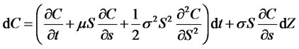 (3)
(3)
 is sufficiently smooth, namely, its secondorder derivatives with respect to S and first-order derivative with respect to t are continuous in the domain. As it can be seen Ito’s lemma, the price change is proportional to a coupled second order partial differential equation which depends on the random stochastic variable
 , the deterministic function
 , and the drift parameter
 . If two people agree on the volatility of an asset they will agree on the value of its derivatives even if they have different estimates of the drift rate.
Replicating the derivative with a stock and a bond First, we form a portfolio using  and
and  so that the portfolio behaves exactly the same with
 . Let’s consider that the portfolio
  consists of
  shares of the stock and
  units of the bond,
 (4)
(4)
We want the portfolio to be self-financing, which means that no money is added or withdrawn. Under this condition, the instantaneous gain in the value of the portfolio due to changes in security prices, by (1) and (2), is
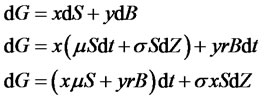 (5)
(5)
In order to mimic ,
,  and
and , that is, (3.5) must coincide with (3.3). Since
  and
and  are independent, the respective coefficients should be equal; otherwise, there will be an opportunity for arbitrage. Therefore, we hope that the following equations will hold
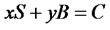 (6)
(6)
 (7)
(7)
 (8)
(8)
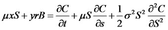
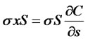
From (8), . Plugging this result into (6), we obtain
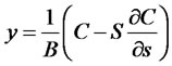 .
.
Plugging these results into (7), we finally obtain
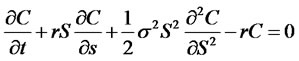 (9)
(9)
This partial differential equation (9) is celebrated BlackScholes equation. In this derivation, we replicated the derivative with a stock and a bond.
Although the exact solution of the Black-Scholes equation is known, a numerical method is so useful. A reason is to create a general numerical model for many different types of options. In particular, American options are not solvable in an analytic sense. If the numerical method works for European style option, then this is the basis to get the solution for an American option [11-13].
Consider a general form of a parabolic partial differenttial equation with non-constant coefficients, Dirichlet boundary conditions and an initial condition (for more details refer to [14]):
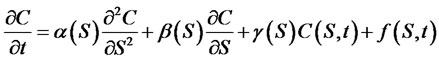 (10)
(10)
Along with boundary and initial conditions
 (11)
(11)
 (12)
(12)
 (13)
(13)
These equations are solved numerically on a grid with N points and a constant step size h. Such a grid is called an equidistant grid. If the interval will be , then the step size is equal to
 . Let each point
  be denoted by
  [19].
[19].
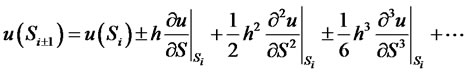
To get a second order central difference approximation of the solution at point , Taylor expansions of the solution in the adjacent points are needed. Applying Taylor’s expansions in the points
  gives:
 (14)
(14)
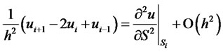
assuming that all relevant derivatives occurring exist. With linear combinations of u at point , it is easily possible to get second order approximations of the first and second derivatives:
 (15)
(15)
 (16)
(16)
here,  is the abbreviation for
 . It is then possible to discretize the differential equation (10). The factors in front of the differential operator can be evaluated in each point xi. For the second order approximation, the semi-discretized systems turn into:
 (17)
(17)
These equations hold for . The first and last point of the system need special treatment. System of equation (34) reads in matrix form
 (18)
(18)
with  is the discretized source function,
  the coefficient matrix and
  the discrete solution. The vector
  contains the boundary values and may be a time-dependent function (see [14] for details) where
  and
and .
.
 (17)
(17)
and the matrix elements read:
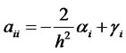 (18)
(18)
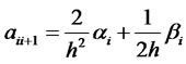 (19)
(19)
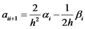 (20)
(20)
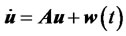
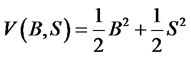
After the space discretization of the equation, which may have been transformed, a system of ordinary differential equations remains
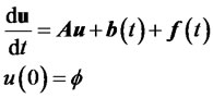 (21)
(21)
with  the matrix generated by the second or the fourth order scheme, the vector
  contains boundary conditions.
  is the source function and
  the (transformed) initial condition (13).
3. Financial Derivatives Drift
Recall now the quantitized financial derivatives equation (35) and modify it in the form
 (22)
(22)
such that
The financial derivatives dynamics (22) represents an affine system (in the input ) which does not have any equilibrium point due to the non-zero drift vector term
  which characterizes a kinematic constraint. Remember that
  term can be treated as an enforced input to the financial derivative system resulted from boundary conditions defined in (17). With zero boundary conditions in Equation (22) yields
 (23)
(23)
which represents a Pfaffian differential constraints (see [20] for Pfaffian differential constraints) but not of kinematic nature arises from the conservation of non-zero financial derivatives.
The transformed financial derivative system (23) can be re-expressed as
 (24)
(24)
System (24) represents a drifted financial derivative system with a drift term d. In such a system the derivative value  can be solved by computing the pseudoinversion
  of the positive definite matrix
  expressed as follows
 (25)
(25)
in which
 (26)
(26)
The financial system (22) is controllable if, for any choice of ,
,  , there exists a finite time T and an input
  such that
 . Unfortunately, general criteria for verifying this natural form of controllability do no exist.
For the sake of the current objective clarification, combine Equations (24) and (25) as a deterministic linear financial system ( ) defined by
 (27)
(27)
The deterministic financial system (28) is composed of bond and stock option experiences a drifted constraint with no equilibrium states. The only possibility of brining such a system to a driftless equilibrium posture to enforce zero risk-free rate  and zero drift parameter
 .
.
Given a neighborhood  of
of , denote by
  the set of states
  for which there exists
  such that
  and
and  for
for . In words,
  is the set of states reachable at time
  from
from  with trajectories contained in V [20]. Also, define
 which is the set of states reachable within time
  from
from  with trajectories contained in the neighborhood
  .
.
The financial system (22) is called:
1) Locally accessible from  if, for all neighborhoods
  of
of  and all
 ,
,  contains a non-empty open set Ω;
2) Small-time locally controllable from  if, for all neighborhoods
  of
of  and all
 ,
,  contains a non-empty neighborhood of x0.
Note that:
• The previous definitions are local in nature. They may be globalized by saying that system (22) is locally accessible, or small-time locally controllable, if it is such for any  in all
 .
.
• Small-time local controllability implies local accessibility as well as controllability, while local accessibility does not imply controllability in general, as shown by the previous example. However, if no drift vector is present, then local accessibility implies controllability.
• However, when dealing with the control of financial systems with generalized Pfaffian constraints, the presence of a drift term  implies that accessibility is not equivalent to controllability.
• For the linearized case of the financial derivative (22), all the previous definitions are global and collapse into the classical linear controllability concept. In particular, the accessibility rank condition at  corresponds to

the well-known Kalman necessary and sufficient condition for controllability as will be detailed in the next section.
A major concern to seek whether financial derivatives can be controlled and if yes, what are the tools to achieve such an objective.
4. Controlability and Observability of Financial Derivatives
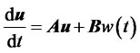
A system is said to be controllable at time  if it is possible by means of unconstrained control vector to transfer the system from an initial state
  to any other state in a finite interval time. The concepts of controllability and observability were introduced by Kalman. They play an important role in the design of control systems in state space. In fact, the conditions of controllability and observability may govern the existence of a complete solution to the control system design. Although most physical systems are controllable and observable, corresponding mathematical models may not possess the property of controllability and observability. In what follows, we shall derive the condition for complete state controllability.
Consider the continuous-time systems shown in Figure 1.
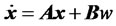 (28)
(28)
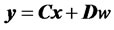 (29)
(29)
where,
 is a state vector
 is
is  -output vector
 is a control signal
 is
is  matrix
 is
is  matrix
 is
is  matrix The system described in Equation (28) is said to be state controllable at
  if it is possible to construct an unconstrained control signal that will transfer an initial state to any final state in a finite time interval
 . If every state is controllable, then the system is said to be completely state controllable [21]. The system is said to be controllable if and only if the following
  matrix is full rank
 .
.
 (29)
(29)
This matrix is called the controllability matrix. A system is said to be observable at time , if with the system in state
 , it is possible to determine its state from the observation of the output over a finite time interval.
The concept of observability is very important because, in practice, the difficulty is encountered with state feedback control is that some of the state variables are not accessible for direct measurement, with the result that it becomes necessary to estimate the unmeasurable state variables in order to construct the control signals. The system is said to be observable if and only if the following  matrix is of full rank
 (30)
(30)
Matrix (30) is commonly called observability matrix.
This following analysis presents a design method commonly called the pole-placement technique. We assume that all state variables are measureable and are available for feedback. It is shown that if the system considered is completely state controllable, then poles of the closedloop system may be placed at any desired locations by means of state feedback through an appropriate state feedback gain matrix as displayed in Figure 2. Let us assume the desired closed-poles are to be at ,
,  , ···,
 .
.
We shall choose the control signal to be
 (31)
(31)
This means that the control signal is determined by an instantaneous state. Such a scheme is called state feedback. The  matrix
  is called the state feedback gain matrix. Substituting (31) into Equation (83) gives
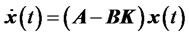 (32)
(32)
The solution of this equation is give by
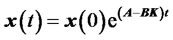 (33)
(33)
where is the initial state caused by external disturbances. The stability and transient response characteristics are determined by the egienvalues of matrix . If matrix
  is chosen properly, the matrix
  can be made asymptotically stable matrix.
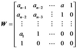
Define a transformation matrix  by
by
 (34)
(34)
where  is the controllability matrix
 (35)
(35)
and
 (36)
(36)
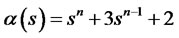
where the  are the coefficients of the characteristic polynomial
 (37)
(37)
Let us choose a set desired egienvalues as ,
, . Then the desired characteristic equation becomes
 (38)
(38)
The sufficient condition that the system to be completely controllable with all egienvalues arbitrarily placed by choosing the gain matrix
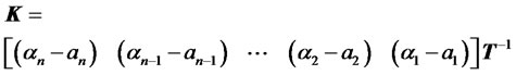 (39)
(39)
Example: Controllability, Observability, State Feedback Control
Let us consider the deterministic Bond-Stock Option dynamics defined in (27) with risk-free rate  and drift parameter
 .
.
For the sake of financial system control we assume the system has been modified such that
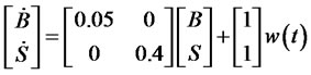
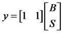
It is desired to check the controllability condition (29) and observability condition (30). It can be easily validated the both controllability matrix and observability matrix are identical  and are of full rank 2.
The original system has two eigenvalues of ,
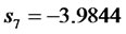
,  , ···. It is desired now to stabilize the system with placing the poles at
 ,
, . Since the system is controllable the pole placement design can be implemented. Then the original and desired characteristic equations are, respectively, given as

The transformation matrix T for the system is
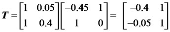
The sufficient condition that the system to be completely controllable with all egienvalues arbitrarily placed by choosing the gain matrix as

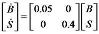
For a negative feedback controlled financial system as shown in Figure 2, it implies that to stabilize such a system, the bonds risk-free rate  should be increased by 6.15 times (from 0.05 to 0.3075) and drift parameter
  should decreased the stock by 9.6 times (from 0.4 to −3.84). From physical point of view, the negative sigh is to balance the increase of the bonds and comply with the conservation of financial money.
Some systems reveal a conservation nature such as mechanical systems which comply with the principle of conservation energy. Liapunov methodology technique utilizes the concept of quadratic function to prove if a given system can be stabilized or not. It is desired to seek such a property in the financial systems as presented below.
5. Liapunov Stability of Financial Derivatives
The template is designed so that author affiliations are

Figure 1. Open-loop financial controlled system.
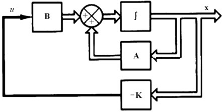
Figure 2. Closed-loop controlled financial system with w = −Kx.
not repeated each time for multiple authors of the same affiliation. Please keep your affiliations as succinct as possible (for example, do NOT post your job titles, positions, academic degrees, zip codes, names of building/ street/district/province/state, etc.). This template was designed for two affiliations. The objective in this section is to investigate the stability of financial systems using Liapunov stability techniques. Consider a reduced dynamics model (28) given by
 (40)
(40)
We assume that  is non-singular. Then the only equilibrium state is the origin
 . The stability of the equilibrium of state of the linear, time-variant system can be investigated by the use of the second method of Laipunov.
For the system defined by (40), let us choose a Liapunov candidate function as
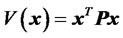 (41)
(41)
where  is a positive-definite function real matrix. The time derivative of
  along any trajectory is
 (42)
(42)
By rearrangement terms
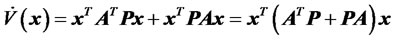 (43)
(43)
Since  is chosen to be, we require, for asymptotic stability, that positive-definite
  be negative definite. Therefore, we require that
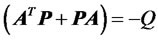
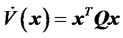 (44)
(44)
where
 (45)
(45)
Example: Liapunov Stability
Let us consider the deterministic Bond-Stock Option dynamics defined in (27) with risk-free rate  and drift parameter
 .
.

It is clear that the equilibrium state is the origin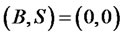 .
.
Let us assume a tentative Liapunov function

where  is to be determined from
The last equation can be written as

or
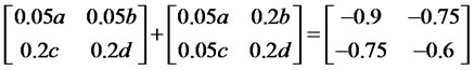
Rearranging corresponding terms leads to

Equating both sides yields to

By then the candidate matrix  is given by
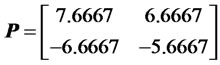
Although matrix  is positive definite positive (its eigenvalues are 1 and 1), but it has not guaranteed the system stability. That is because the time derivative of the Liapunov candidate
  is increasing, since
  has positive egienvalues (2.2948 and 0.0002). Such a stock-bond system behaves like an unstable node at the origin as shown in Figure 3.
Former analysis can be summarized in the following theorem.
Theorem: Consider the financial dynamic system described by , where
  is an
is an  state vector and
  is
is  constant nonsingular matrix. A necessary and sufficient condition that the equilibrium state
  be asymptotically stable in large is that, given any positive-definite real matrix
 , there exist a positive-definite real matrix
  such that
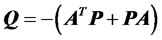
The scalar function 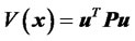 is Liapunov candi-
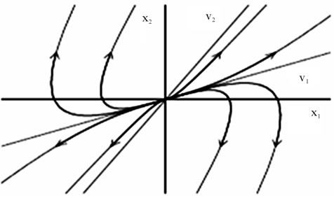
Figure 3. Bond-stock unstable node at the origin.
date function for this system.
Example
To illustrate such a concept let us consider a financial system composed of a bond  and a stock
  described by
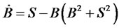 (46)
(46)
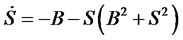 (47)
(47)
Cleary, the origin 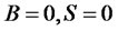 is the only equilibrium state. Determine now its stability. Let us define a financial scalar function
 (48)
(48)
which is positive definite, then the time derivative of  along any trajectory is
 (49)
(49)
which is negative definite. This shows that  is continually decreasing along any trajectory; hence
  is a Liapunov function that guarantees the equilibrium state at the origin of the financial system is asymptotically stable in large as shown in Figure 4.
Such a candidate function (48) characterizes the conservation of the financial system (similar to the principle of conservation of energy). The bond-stock dynamics (46) and (47) characterizes also that it is not possible that both are increasing. That is due to the fact that both are conserved and have constant values. Truly, if for example the bond is increasing, then the stock should be decreasing.
6. Controlled Financial Derivatives System
There are two types: component heads and text heads. For the sake of testing the controllability of Black-Scho-

Figure 4. Stability of the stock-bond system.
les Derivatives Formula recall the disrcretized form in Equation (16) assuming zero source function  as follows
Assuming risk-free rate , variance
  and for 6 months, with constant left boundary condition
  and constant right boundary conditions
  with a step size of 0.1.
where the coefficient matrix
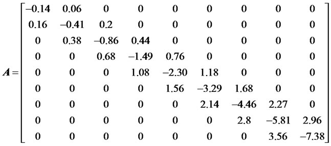
and the input vector is
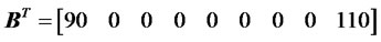 ;
;
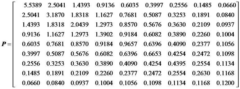
We are seeking a Liapunov candidate function that satisfies conditions (41), (44) and (45), such that

It is possible to start with appositive definite matrix  to serve this goal. Performing calculations leads to the following definite positive matrix:
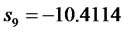
It is desired now to design a state-feedback financial controlled system such that the desired closed loop poles are:
 ,
,  ,
,  ,
,
 ,
,  ,
,  ,
,
 ,
,  ,
, .
.
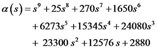
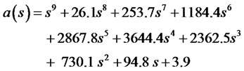
With a corresponding characteristic equation
Compared to the original eigenvalues (poles):
 ,
,  ,
,  ,
,
 ,
,  ,
,  ,
,
 ,
,  ,
, 
with characteristic equation is given by:
Before proceeding it is crucially important to check the controllability and observability conditions (29) and (30). Mathematical implementations provide that the controllability matrix and observability matrix are both of full rank 9. It implies that we can design a pole placement controller at any desired location.

Gain calculations based on Equation (37) yields to the following values (in Millions)
 (in Millions)
The results show that in order to guarantee the stability of financials systems at the origin with the desired poles it is necessary to provide a negative feedback gain as shown in the former gain vector. It implies that for the first option  the output value should be magnified as 83.5 times the financial output 1 (in Millions)
580.4 times the financial output 2 (in Millions)
1291.1 times the financial output 3 (in Millions)
1501.2 times the financial output 4 (in Millions)
967.2 times the financial output 5 (in Millions)
351.2 times the financial output 6 (in Millions)
69.8 times the financial output 7 (in Millions)
6.9 times the financial output 8 (in Millions)
0.3 times the financial output 9 (in Millions)
From practical point of view, it means that to keep the financial derivative system stable, $83.5 millions times the financial output1 must be injected into the financial system under consideration. Simulation results shown in figure 5 show that the financial derivative system has been brought back to its equilibrium state. This explains the inflation and financial derivatives deficit.
The transformation of the financial derivative system into heat equation is demonstrated in Figure 6. Such results verify the stability of the system as well. In the simulation it is assumed a non-constant heat coefficient exponentially decreasing.
7. Conclusions
Just Recently the Global Financial Economy has been suffering from the worst financial crisis since the Great Depression sicne 1930. The current crisis is triggered by the shortfall of liquidity in the United States, followed by collapsing of large financial institutions, bailout of banks, turndowns of international stock markets and credits, collapse of housing bubble, mortgage foreclosures, failure of key businesses, declines of wealth, increase of governmental debts due to substational commitments.
Financial derivatives are blamed for the catastrophic financial crisis since 1997. The Bank of International Settlements (BIS) in Switzerland has recently reported that global outstanding derivatives have reached 1.14 quadrillion dollars: $548 Trillion in listed credit derivatives plus $596 trillion in notional OTC derivatives. Many experts claim that the core theories/theorems were based on wildly unrealistic assumptions and did not stand out for their empirical strength. This view led to a series of financial practices that increased the fragility and vulnerability of financial institutions setting the context for the occurrence of financial crises including the current one.
Equilibrium, stability and control of financial derivatives is the concern of this article. Such objectives are investigated based on the descertization of Balck-Scholes formula to a system of linear ordinary differential equations.
It is figured that such Black-Scholes based financial derivatives experience a drift which hardly can be brought to equilibrium state. The financial derivatives dynamics represents an affine system which does not have any equilibrium point due to the non-zero drift vector term which characterizes a kinematic constraint.
Conditions of controllability and observability of financial systems are introduced. Moreover, stability of such derivatives is tested by the virtue of Liapunov methodology. It is proved that financial system should satisfy the quadratic form which can be interpreted as conservation of financial instruments. This candidate inherits the conservation of physical money.
For Bond-Stock option it is implied that to stabilize such a system, the bonds risk-free rate  should be increased and drift parameter
  should decreased the stock. From physical point of view, the negative sigh is to balance the increase of the bonds and comply with the conservation of financial money.
Such a candidate function for stock-bond option is proposed. It characterizes the conservation of the financial system (similar to the principle of conservation of

Figure 5. Financial derivatives controlled system.

Figure 6. Financial derivatives in the heat transformed form.
energy). The bond-stock dynamics reveals that it is no t possible that both are increasing. That is due to the fact that both are conserved and have constant values. Truly, if for example the bond is increasing, then the stock should be decreasing.
Furthermore, a financial state-feedback control system is proposed. Such analysis shows that the financial derivatives system needs to be injected with cash to maintain a stable financial system. These results can explain the shortfall of liquidity needed to substitute for the 1.14 quadrillion dollars bubble. Finally, scenarios and simulation are demonstrated to verify the effectiveness of the proposed approach.
The results show that in order to guarantee the stability of financials systems at the origin with the desired poles it is necessary to provide a negative feedback gain as shown in the former gain vector. From practical point of view, it means that to keep the financial derivative system stable, liquidity must be injected into the financial system under consideration. Simulation results shown in figure show that the financial derivative system has been brought back to its equilibrium state.
Future work will focus on how a financial derivative system can be controlled by designing an observer (estimator) without the need of measuring all derivatives values.
REFERENCES
- Monetary and Economic Department, “OTC Derivatives Market Activity in the Second Half of 2008,” Bank for International Settlements, Basel, 2009.
- M. Shibli, “The Fundamental Principle of Conservation of Physical Money: Its Violation and the Global Financial System Collapse,” Journal of iBusiness, Vol. 3, No. 1, 2011, pp. 76-87. doi:10.4236/ib.2011.31013
- K. Schwab, “The Future of the Global Financial System: A Near-Term Outlook and Long-Term Scenarios,” World Economic Forum’s World Scenarios Series, 2009.
- P. Krugman, “How Did Economists Get It So Wrong?” New York Times, 2009.
- E. P. Caldentey and M. Vernengo, “Modern Finance, Methodology and the Global Crisis,” Real-World Economics Review, No. 52, 2010, pp. 69-81.
- Wharton School of the University of Pennsylvania, “Why Economists Failed to Predict the Financial Crisis,” Knowledge@Wharton, 2009. http://knowledge.wharton.upenn.edu/article.cfm?articleid=2234
- F. Black and M. Scholes, “The Pricing of Options and Corporate Liabilities,” Journal of Political Economic, Vol. 81, No. 3, 1973, pp. 637-654. doi:10.1086/260062
- J. Hull, “Options, Futures and Other Derivatives,” 5th Edition, Prentice Hall, Upper Saddle River, 2003.
- Ö. Ugur, “An Introduction to Computational Finance,” World Scientific Publishing, Singapor, 2008.
- H. Lee and D. Sheen, “Laplace Transformation Method for the Blck-Scholes Equation,” International Journal of Numerical Analysis and Modeling, Vol. 6, No. 4, 2009, pp. 642-658.
- C. C. W. Leentvaar and C. W. Oosterlee, “Multi-Asset Option Pricing Using a Parallel Fourier-Based Technique,” Journal of Computational and Applied Mathematics, Vol. 222, No. 1, 2009, pp.193-209. doi:10.1016/j.cam.2007.10.015
- C. W. Oosterlee, “American Options with Discrete Dividends Solved by Highly Accurate Discretizations,” Mathematics in Industry, Vol. 8, Part 7, 2006, pp. 427-431.
- C. W. Oosterlee, C. C. W. Leentvaar and A. A. Vazquez, “Pricing Options with Dividends by High Order Finite Difference and Grid Stretching,” European Congress on Computational Methods in Applied Sciences and Engineering (ECCOMAS), 2004.
- C. C. W. Leentvaar, “Numerical Solution of the BlackScholes Equation with a Small Number of Grid Points,” Master’s Thesis, Delft University of Technology, Delft, 2003.
- Y. Y. Ye, “A Path to the Arrow-Debreu Competitive Market Equilibrium,” Journal of Math Programming, Vol. 111, No. 1-2, 2006, pp. 315-348. doi:10.1007/s10107-006-0065-5
- Robert Almgren, “Financial Derivatives and Partial Differential Equations,” American Mathematical Monthly, Vol. 109, 2001, pp. 1-12. doi:10.2307/2695763
- K. J. Arrow and J. Debreu, “Existence of an Equilibrium for a Competitive Economy,” Journal of Econometric Society, Vol. 22, No. 3, 1954, pp. 265-290.
- K. J. Arrow and M. McManus, “A Not on Dynamic Stability,” North-Holland Publishing, Amsterdam, 1958.
- G. W. Recktenwald, “Finite-Difference Approximations to the Heat Equation,” Class Notes, 2004.
- De Luca and G. Oriolo, “Modeling and Control of Nonholonomic Mechanical Systems,” In: J. A. Kecskemethy, Ed., Kinematics and Dynamics of Multi-Body Systems, CISM Courses and Lectures, No. 360, Springer-Verlag, New York, 1995, pp. 277-342.
- K. Ogata, “Modern Control Engineering,” Prentice Hall, Upper Saddle River, 1997.