Journal of Electromagnetic Analysis and Applications
Vol.4 No.6(2012), Article ID:20340,5 pages DOI:10.4236/jemaa.2012.46036
Decagon Charged Pendula and Beyond
![]()
Department of Physics, Pennsylvania State University, York, USA.
Email: has2@psu.edu
Received April 20th, 2012; revised May 19th, 2012; accepted May 27th, 2012
Keywords: Electrostatic Interaction; Mathematica
ABSTRACT
We consider a set of n identical charged pendulums and hang them from a common pivot. The electrostatic repulsive charge-charge interaction between the pairs repels the pendulums apart. The weight and the tension of the pendulums balance the coulombian repulsion stabilizing the setup to final static equilibrium. The final configuration is a horizontal n-gon inscribed in a circle of radius, R. It is the objective of our investigation to measure R as a function of mass, length and charge, {m, ,q}, of the pendulum for a number of pendulums, n, within the range of 2 ≤ n < ∞. As a by-product of the analysis for a chosen, n, we evaluate the tensions in the lines.
1. Motivations and Goals
It is the objective of our investigation to quantify the impact of two-body coulombian electrostatic interaction [1] to an assembly of limitless number of identical charges. We begin with an assembly of two-charged particles and systematically generalize the analysis by increasing the number of the particles. In order to quantify the impact of the electrostatic forces we consider static scenarios. For instance we envision utilizing the charges forming identical simple pendulums and hanging them from a common pivot. The pendulums lines confine the movement of the charges. Active forces on the particles including gravity results in equilibrium, bringing the assembly to its final rested configuration. The generalization of the analysis embodies a calculation addressing the quantification of the electrostatic forces transiting from a discrete charge distribution to the continuum. Aside from the physics content of the project at hand, the premise of the project is to exercise applying cutting-edge emerging Computational Algebra System (CAS) in general and Mathematica [2] in particular to physics. The testimonial of the latter is the fabrication of this entire manuscript in one single file embodying text, graphics, simulation, numeric and symbolic computations. This work is composed of four sections. In addition to Motivation and Goals, in Section 2, we lay the fundamentals of the needed physics. In this section we also present the numeric output of the calculation. In Section 3 we present the calculation concerning the continuous charge distribution and compare its numeric values to its discrete counterpart. We close the article with a few closing remarks.
2. Fundamentals and the Physics of the Problem
We begin our analysis considering three charges. Figure 1 depicts one such setup. Each of the three massive charges form a simple pendulum and all three are hooked at a common pivot at a support. The repulsive coulombian forces repel the charges. Each charge experiences a pair of electrostatic force. One such force acting on charge 1 due to charge 2 is denoted by F21. The orientation of the second electrostatic force, F31, is shown as well. The orientation of the net force acting on charge 1 aligns along the extension of the radius of a virtual circle shown by the solid line. At static state this force balances out with the horizontal shadow of the tension in the line. The equal characters of the three pendulums namely, mass, length, and charge, {m, ,q} put the charges evenly in the shown horizontal dashed circle of radius, R.
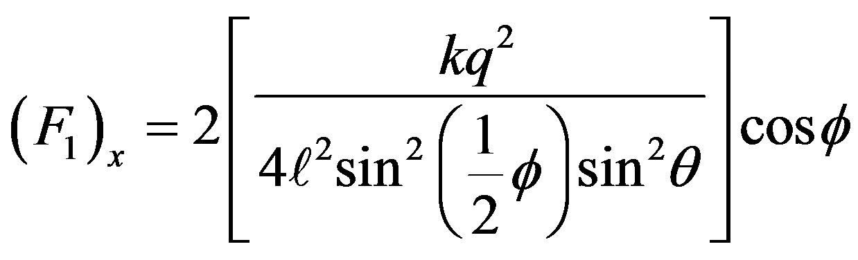
In order to establish the relationship between the relevant physical and geometrical quantities, we begin with the static requirement, . In a 2-dimensional horizontal coordinate system laid on the horizontal circle shown in Figure 1, with the origin at the center of the circle and with x-axis along the radius of the circle, the static force equation yields,
 (1)
(1)
where the coulombian forces,  with
with ,
,  and {x1,y1} = {R,0} with
 . In MKS units the
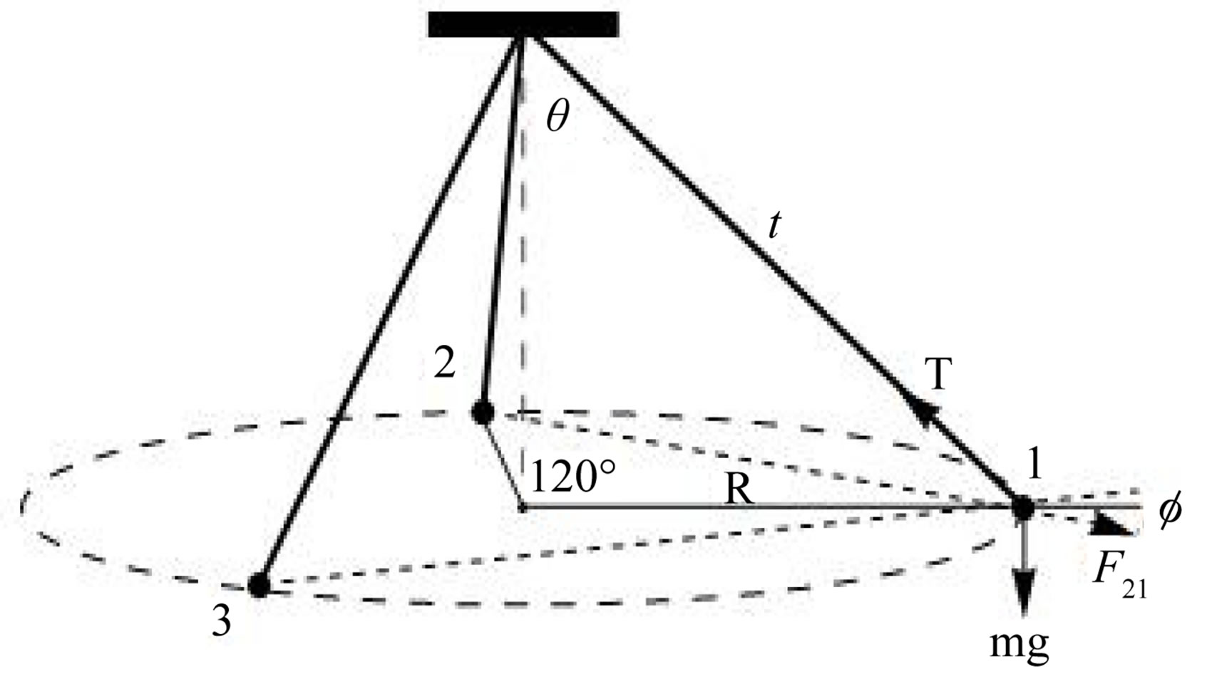
Figure 1. Three-pendula setup. The relevant forces, weight, tension and one of the electrostatic forces are shown.
value of  and q is in coulombs. Substituting these polar coordinates in r21 yields,
 . On the other hand in the upright traingle shown in Figure 1 we have
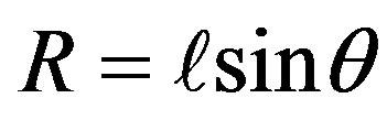 , where
  is the “conic” angle, the angle the string makes with the vertical dashed reference line. Putting these together gives,
 (2)
(2)
This force needs to be balanced with the horizontal component of the tension. The weight counter balances the vertical component of the tension. These two requirements yield,
 (3)
(3)
Forming the ratio of these two equations and substituting for Equation (2), gives,
 (4)
(4)
In Equation (4) we utilize the trigonometry identity, sin2θ = tan2θ/(1+tan2θ), this yields,
 (5)
(5)
where
 (6)
(6)
The subscript 3 indicates the number of the charges. At the outset for a chosen set of parameters, {m, ,q}, solution of cubic Equation (5) gives the conic angle θ. Utilizing this angle the radius of the circumscribed circle R is determined.
Utilizing the result of the three-charge system we systematically extend the analysis for a system of n charges. The virtual circles formed by the charges for 2 ≤ n ≤ 7 are shown in Figure 2. The middle graph of the first row
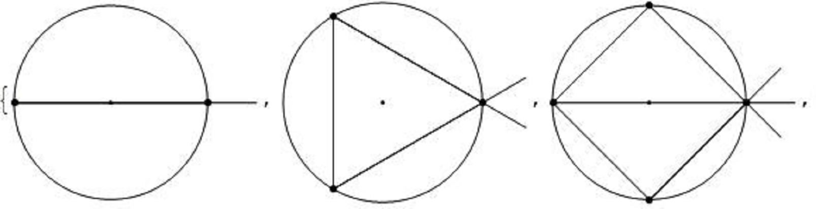
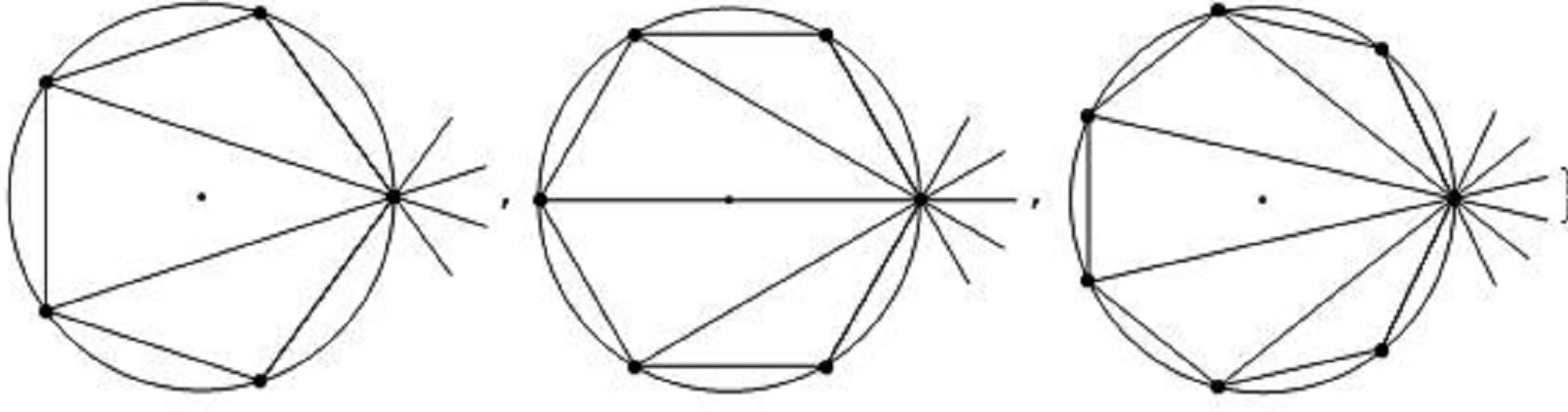
Figure 2. Self-organized distributed point-like charges for n = 2, 3, 4··· 7.
corresponds to the calculation presented thus far. Utilizing these graphs the distance between the far right charge and the rest of the charges are calculated. These figures are also used to calculate the needed angles for evaluating the horizontal components of coulombian forces. Plots depicted in Figure 2 reveal the fact that configuration of the distributed charges for even and odd charges are different. In both cases the distributions possess symmetry about the horizontal axis that passes through the center of the circle. However, for even number of charges there is always one purely horizontal coulombian force originating from the far left charge; this is missing for the odd cases. Consequently, the format of the net force for even number of charges is different from the odd cases. However, one realizes A3 given by Equation (6) is composed of two distinct terms; the physical quantities are lumped together in the first parentheses, while the second parentheses contains the angular terms of the associated geometry. Therefore, n > 3 changes only the value of the second parentheses. Utilizing the symbolic computational features of Mathematica for a chosen number of charges, n, the second column of Table 1 gives the terms of the second parentheses for An. The third column of the same table is the associated numeric values of the second column.
Inspection of this table confirms the comments made in the previous paragraph. Namely, the common value 1/2 for even n’s is the signature of the far left charge; this factor is absent for the odd n’s. In Table 1, because of space limitation only the terms for the 10-charge configuration, the decagon, are given. With no restriction the table can be extended for a limitless number of charges, i.e. 2 ≤ n < ∞.
Utilizing the terms given in Table 1 and adopting the format of Equation (5) we compose the general equation for a n-charge system, namely,
 (7)
(7)
 (8)
(8)
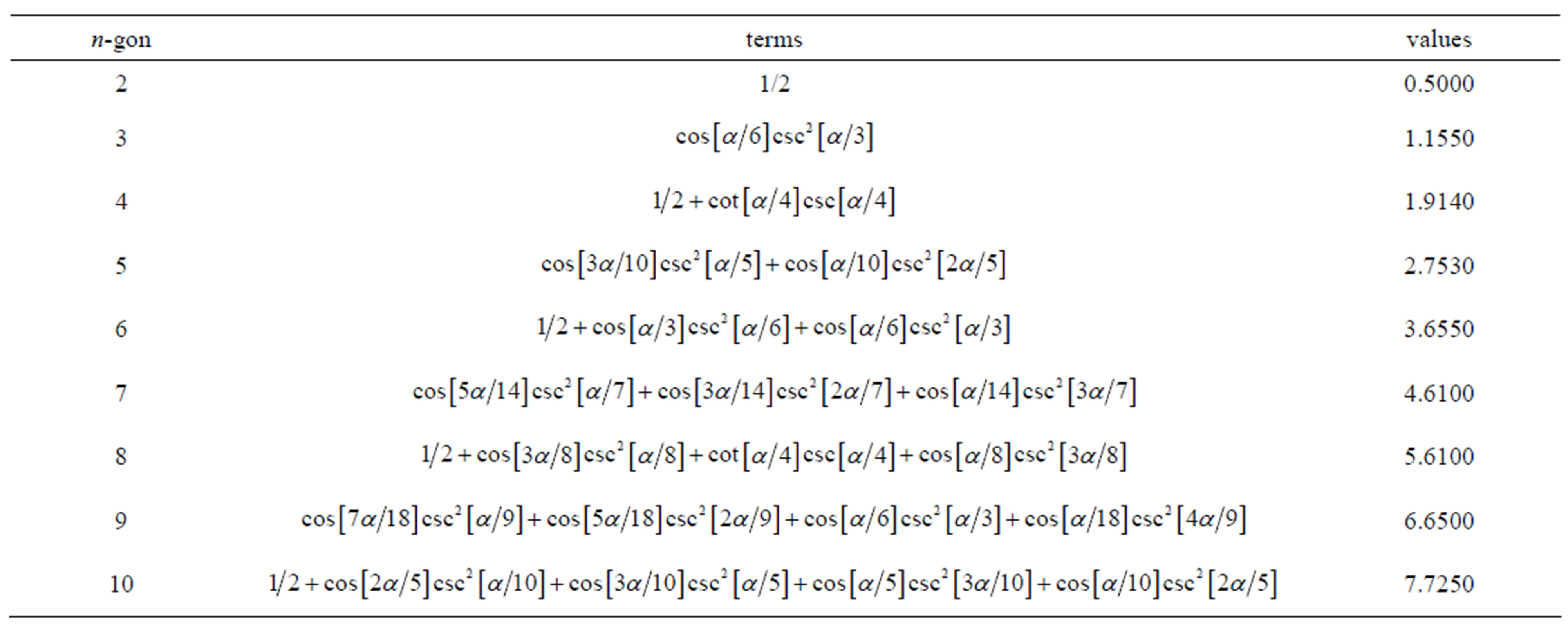
Table 1. The first column is the number of charges, the second column is the symbolic geometry related factor of corresponding, An, and the third column is the numeric values of the 2nd column for α = π.
For a set of reasonable values of {m, ,q} such as {m→1·10–6, q→5·10–9,
  →1.0} in metric units we evaluate An. Deploying Mathematica numeric equation solver we then solve Equation (7) for θn. With these roots at hand 1) we plot the conic angle θn vs. n, and 2) applying Rn =
  sinθn we evaluate and then display the radii of the virtual circles in Figure 2. Finally according to Equation (3), Tn cosθn = m·g we display the tension in the pendulum vs. n. These are shown in the graphic matrix, Figure 3.
As mentioned earlier, Table 1 contains the terms associated with 2 ≤ n ≤ 10. Plots depicted in Figure 3 are those for 2 ≤ n ≤ 32. It is interesting to observe that the angle θn and the radii Rn are not linear functions of n, where the tension behaves linearly. Interested observers may verify objectively the impact of varying the characters of the pendulums on the shown plots of Figure 3. For instance one should expect a larger charge q results in a larger angular variation. On the contrary a heavier mass m results in a smaller angular deviation vs. n, and etc.
3. Continuous Charge Distribution
As show in Figure 3 increasing the number of charges increases the radii of corresponding virtual circles accordingly. As shown, the radius is not a linear function of n. For large n the rate of change of R is drastically milder vs. its rate for the smaller n. The consequence of this observation is that the distance between the adjacent charges for instance for a decagon is 0.27 m where for a set of 30 charges it is 0.13 m, i.e. it is half as large. In other words, the distribution of a large number of charges may be considered to be approaching to continuum. Therefore, we consider a “large” number n as a continuous distribution and evaluate the force that such distribution exerts on a single charge placed on the plane of the circle. The strategy is to apply , where
 , the electrostatic potential is subject to the density of the continuous charge distribution, λ = (n·q)/(2π·R). The integration yielding the potential is,
 (9)
(9)
where, R is the radius of the loop, x, is the distance of a point from the center of the loop along the x-axis in the coordinate system used throughout this article, and  is the angle between the radius vector connecting the center of the loop to a point on the rim of the loop and the x-axis. Since for the case at hand
 , Fx is,
 (10)
(10)
 (11)
(11)
EllipticK, and EllipticE are the elliptic integral of the first and the second kind, respectively [3]. It might be tempting to evaluate the electric field directly by integrating the square of the denominator of the integrand in Equation (9); however, this increases the CPU time dras-
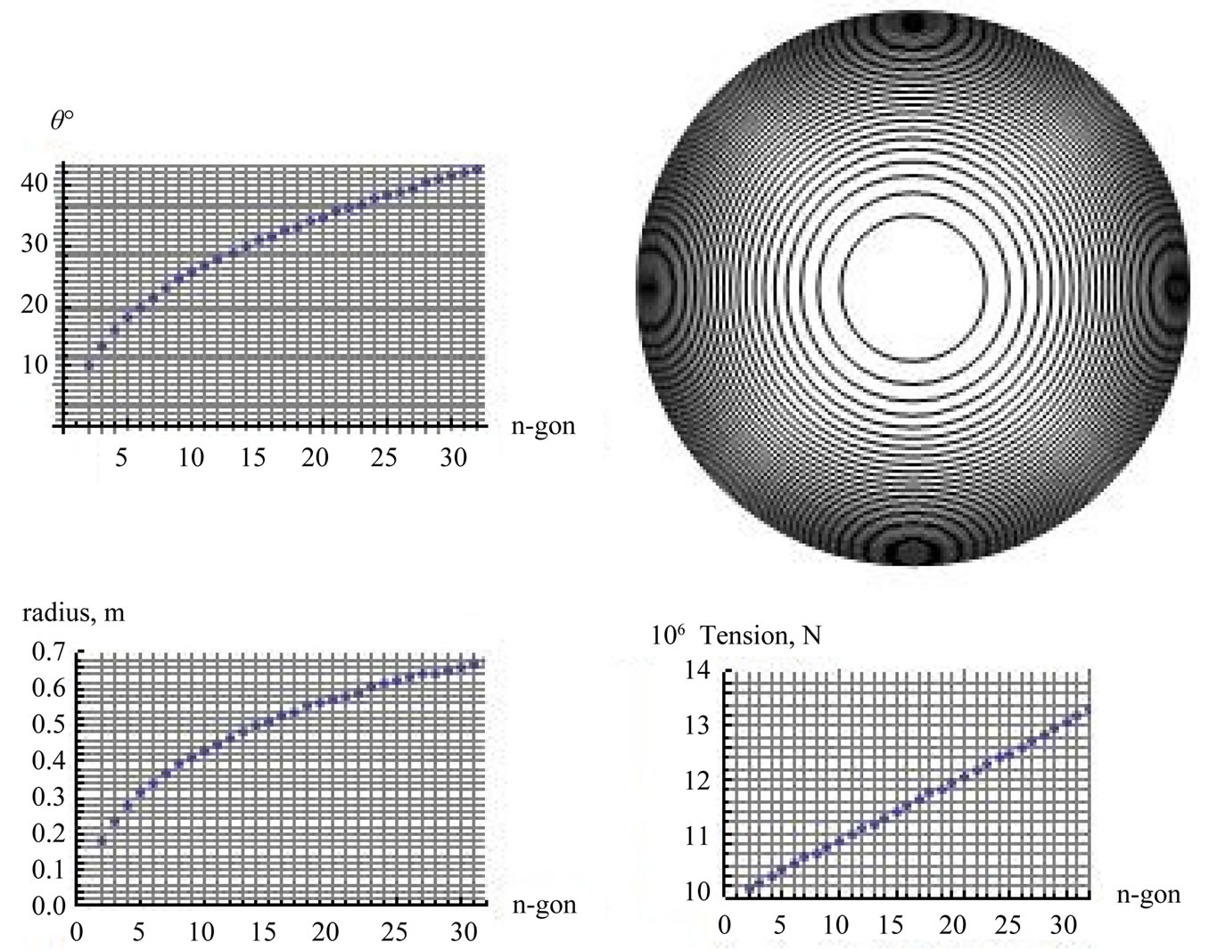
Figure 3. The left upper graph is the display of the conic angle θn vs. n. The right upper graph is the display of the corresponding circular orbits. The bottom two graphs are Rn and Tn vs. n.
tically. The proposed strategy is preferred.
We then for instance compare the numeric value of Equation (11) for n = 32 to the force value according to the modified version of Equation (2), i.e.
 .
.
In order to match these two forces we realize the radius, R, in the former needs to be about (20-30)% greater than the values used in the latter. The value of x also is to be about 50% - 60% greater than the radius R. In other words, there is no unique set of values {R,x} that is conducive to the matching values of these two forces. For the chosen finite number of charges, n, one might interpret the required larger radius corresponds to the needed thinner (discrete) charge distribution.
4. Conclusion and Remarks In this article by utilizing the fundamentals of a two-body static electrostatic interaction we consider a controlled situation where n charges are present. By restricting the movement of the charges we envision a situation where the charges organize themselves forming various two dimensional n-gons. We then evaluate the coulombian forces of the n – 1 charges on one of the charges. Evaluation of this force entails calculating certain projection angles. In the course of analyzing these forces we were able to recognize a certain pattern conducive to formulating the problem for a limitless number of countable charges. Due to space limitation we report the general trend of a decagon. However, in the course of numeric analysis we use the extended version of the pattern evaluating a 32- charged set. With great efforts we developed a Mathematica code automating the evaluation of the symbolic and the corresponding numeric values of terms in Table 1. As pointed out in the Introduction section, we deploy Mathematica utilities crafting the needed graphs, as well as symbolic and numeric evaluations. Furthermore, we also reason that for a large number of charges the distribution appears as continuous. Applying Mathematica symbolic computational power we are able to evaluate symbolically the electrostatic potential, its associated electric field and the force.
5. Acknowledgements
The author is grateful to Mrs. Nenette S. Hickey for her editorial comments. He is also thankful to the anonymous referee for suggesting to augment the investigation by replacing the point-liked charges with finite sized spheres.
REFERENCES
- J. D. Jackson, “Classical Electrodynamics,” 3rd Edition, Wiley, Hoboken, 2005.
- S. Wolfram, “The Mathematica Book,” 5th Edition, Cambridge University Publications, Cambridge, 2003.
- http://mathworld.wolfram.com