Applied Mathematics
Vol. 4 No. 2 (2013) , Article ID: 28191 , 6 pages DOI:10.4236/am.2013.42045
Modeling Population Growth: Exponential and Hyperbolic Modeling
Stanford Educational Program for Gifted Youth, Palo Alto, USA
Email: dhathout@aol.com
Received December 7, 2012; revised January 7, 2013; accepted January 15, 2013
Keywords: Exponential Growth Modeling; Hyperbolic Growth Modeling
ABSTRACT
A standard part of the calculus curriculum is learning exponential growth models. This paper, designed to serve as a teaching aid, extends the standard modeling by showing that simple exponential models, relying on two points to fit parameters do not do a good job in modeling population data of the distant past. Moreover, they provide a constant doubling time. Therefore, the student is introduced to hyperbolic modeling, and it is demonstrated that with only two population data points, an amazing amount of information can be obtained, such as reasonably accurate doubling times that are a function of t, as well as accurate estimates of such entertaining topics as the total number of people that have ever lived on earth.
1. Introduction
This year, the world’s population passed the 7 billion mark. Being able to forecast population in the future, and even being able to answer some interesting questions about population in the past, depends on developing accurate mathematical models of population growth. This model development makes for an excellent calculus project. Here, I present such a project that I think might achieve multiple specific learning objectives in a very step-by-step fashion, and provide students with a genuine feel for how theoretical mathematics has very real-world applications. This project follows the lines developed by Banks [1].
The learning objectives are as follows:
1) Learn to use the wealth of available internet resources, such as Google Data, to obtain information on world population. This involves such simple skills as reading graphs and tables;
2) Learn to plot data, using programs such as Excel;
3) Develop a simple exponential model of population growth by understanding its assumptions and learning how to solve a simple first order differential equation. Learn how to solve for the model’s parameters in a very simple way. In this paper, we use initial values from 1960 and 2009;
4) Compare the model to recent population data, say from the 20th century. The students will see that there is an excellent fit between actual and predicted population values. This will give confidence in using the model to forecast future population growth, e.g., when will the world population reach 10 billion or 100 billion, or what will the population be in 2050?
5) Compare the exponential growth model to more remote population data, starting at 1 AD. Students will then see that there is now a serious discrepancy between the model and actual data, spurring the search for a new model;
6) Students will develop a hyperbolic growth model, as an illustration of modeling using a relative growth rate which is not constant, but is a function of the population. The hyperbolic growth model differential equation is developed and solved, once again estimating parameters in a very hands-on simple fashion. This model is then compared to real data. Students will find a much better fit with past population data. The weaknesses of the hyperbolic model (e.g., it cannot forecast the distant future because of asymptotic behavior) are discussed;
7) Students will develop expressions for doubling times using both models, and learn the difference between a constant doubling time (as in the exponential growth model) and a time-dependent doubling time (as in the hyperbolic growth model);
8) The hyperbolic growth model will be used to answer such interesting questions as, “How many people have lived since the birth of Jesus?” or “Of all the people who have ever lived on earth, what percent are alive today?” Students can test their intuition on the last question before solving for the answer, since there have been specious reports in the media, for example, purporting that of all the people who have ever lived, 75% are alive today, etc.;
9) Students will come to appreciate that different models can be used to describe the same data, each with its own strengths and weaknesses. For example, given only the simple tools of an introductory calculus course, we would rely on an exponential model to forecast future population growth, but on a hyperbolic growth model to answer questions about the past.
To achieve these ends, the paper begins by asking students to collect world population data from 1 AD to the present. Using only two data points, an exponential growth population model is developed and used both to project future population and compare to past population data. A hyperbolic growth model is then developed, and its fits to prior population data are compared with the exponential model. Expressions for doubling times are derived from both models and compared to real world data. Finally, the hyperbolic growth model is used to estimate the number of people that have ever lived on earth. In the conclusion section, the student is pointed to the notion that the simplistic models presented here are insufficient for truly accurate projections, and that such projections would need to take numerous additional factors into account.
2. World Population Data
The first step in developing a population model is to research world population data. Estimates of world population from 1 AD through the present are available from various sources [2,3].
With sufficient data points, a nice graph of world population over time can be produced to allow us to visualize the trend of population growth. We see a very sharp increase starting about 1900 (Figure 1).
3. Mathematical Models
3.1. Exponential Growth Population Model
It is possible to construct an exponential growth model of population, which begins with the assumption that the rate of population growth is proportional to the current population:
where k is the rate of population growth (in yr−1), and P is the population. This differential equation produces a model of the following form:

Using data from two arbitrary sample points, e.g., 1960 and 2009, where the world population was 3.0402 and 6.8158 billion respectively, we can determine C and

Figure 1. World population (in billions) versus time, starting at 1 AD.
k as follows. We set 1960 as the t = 0 time point by recasting the model as follows:

Since in 1960, the population was 3.0402 billion, this makes
 .
.
So, we can write our model as:

Now, using the population data from 2009, we can solve for k as follows:

Thus, the exponential model can be written as:

This model can now be used to make future predictions about the population, as shown in Figure 2:
We see an excellent agreement between actual data and predicted data between 1960 and 2011, and so this gives us some confidence about forecasting the future.
Thus, using our model, we can plug in t = 2050 to estimate the population in that year in billions,
Also, the model can be used to determine the year in which a specific population target will be reached, such as 10 billion or 100 billion. Setting  billion, we get t = 2032.27, so the population is estimated to reach 10 billion during the year 2032. Similarly, the population is estimated to reach 100 billion in the year 2172.
Additionally, we can use the exponential growth model to estimate the rate of growth as follows:
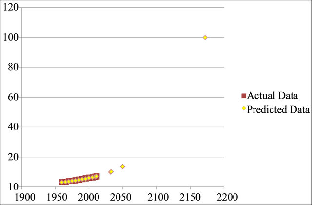
Figure 2. Actual population data (in billions) from 1960 to 2011 versus predicted data using the exponential model, with future population predictions.

gives us
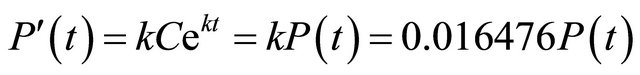 which of course is the differential equation that gives rise to the exponential model. Thus, the rate of population growth at any time, in billions per year, is simply the population at that time multiplied by k, the relative growth rate, which we have already determined. For example, in 2009, P(t) = 6.816 billion, giving us that P’(t) is 0.112 billion/year. This leads to a predicted population of 6.816 + 0.112 billion = 6.928 billion in 2010, which is quite close to the actual figure of 6.8944 billion.
3.2. Comparing the Exponential Growth Model to Real Data
Now that we have our exponential model of population growth, it would be interesting to see how its predictions about the more distant past compare with the true population data, since this is a good way to gauge the accuracy of the model. Using our equation,
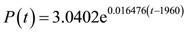
we can calculate what the model would predict about the past (Figure 3):
We see that the exponential model provides an excellent fit for the data beginning about 1950, but significantly underestimates the actual population at earlier times. This makes it interesting to explore other models.
3.3. Developing a New Model: Hyperbolic Growth
With exponential growth, we began with the differential equation,


Figure 3. World population (in billions) versus time, starting at 1 AD. Series 1: actual population data. Series 2: population as predicted by the exponential growth model.
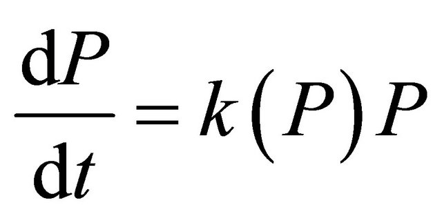
where we assumed that k, the relative growth rate, was a constant. Now, we would like to explore altering this assumption, where in general k becomes a function of P, i.e.,
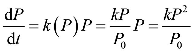
Probably the simplest such function, used in what are called hyperbolic growth models, is to assume that k is proportional to P [4]. This model makes some sense, in that as population grows, this may indicate favorable economic conditions or social conditions which encourage people to have more children, and so the rate of population increase actually grows with the population. To maintain the dimensions in the equation, we can say that

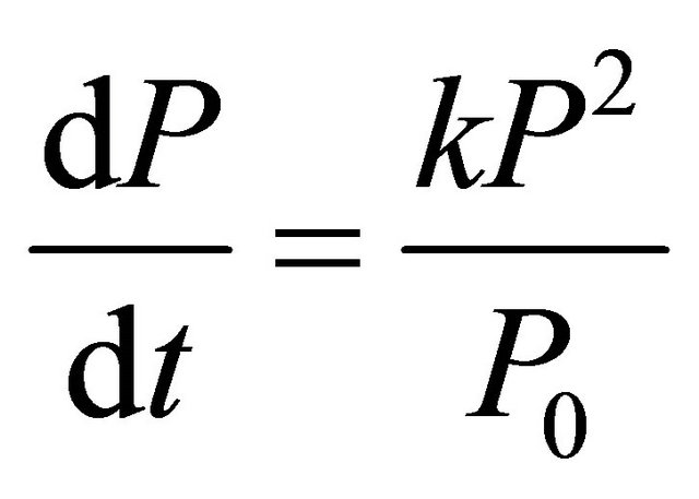
where on the right, k is now a constant multiplied by P, which varies with time, and P0 is a constant. Now, our differential equation becomes:
Now, we need to solve the differential equation,
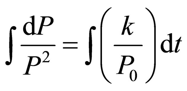
This can be done by separation of variables, so that we have

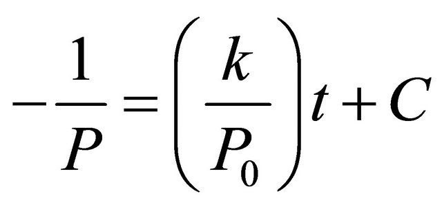
Now, we can integrate both sides, such that
This gives us that
Now, if we say that the population is P0 at time t = 0, then we see that
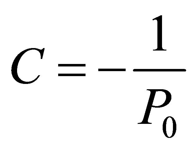
So, we have as our hyperbolic growth model,

Once again, we can use data from 1960 and 2009 to get our constants. We let 1960 be our zero time point, and so , and use this to find k, by manipulating the equation above:
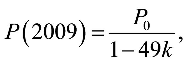
or

Therefore, we can now write our hyperbolic growth model as:
 .
.
3.4. Comparing the Hyperbolic Growth Model to Real Data
Just as we did with the exponential growth model, we can compare our hyperbolic growth model to the real population data we have (Figure 4):
We see that overall, the hyperbolic growth model gives a better fit to the data. To compare this to the exponential model, we can plot the predictions of both models against the real data (Figure 5). We see that
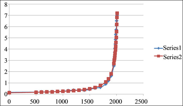
Figure 4. Hyperbolic model versus real data. Series 1: actual population data (billions) versus time. Series 2: predictions of the hyperbolic model.

Figure 5. Real population data (Series 1) versus both the hyperbolic model (Series 2), and the exponential model (Series 3).
overall the hyperbolic model is significantly more accurate for the past, while the exponential model is slightly more accurate for the modern era:
Of course, we have to be very clear that the hyperbolic model, while accurate for the current and past data, has one fatal flaw in terms of future prediction, in that it goes to infinity at 0.0113 (t − 1960) = 1, or t = 2048.5, so it predicts that the population would become infinite in the year 2048!
We see that overall, the hyperbolic growth model gives a better fit to the data.
4. Doubling Times
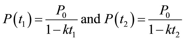
One very interesting issue about populations is how long it takes the population to double, known as the doubling time. We can use both of our models to predict the doubling times. For the exponential model, let us say we observe the population to be  at some point t1, and we want the time interval it takes for the population to double:

Then at time t2, the population has doubled and we have
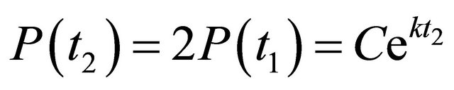
Dividing the second equation by the first, we have

Thus, for the exponential model, the doubling time is a constant, and depends on the value of k.
In our model, k = 0.016476 yr−1, and so the doubling time is about 42 years. This seems to fit pretty well with the modern data, where in 1960, the population was about 3.04 billion people, and in 2000, it was about 6.12 billion people. However, the doubling time given by the exponential model is a constant, and we see that for earlier times, it is not accurate. For example, it took about 150 years for the population to double from 0.61 billion in 1700 to 1.2 billion in 1850. Also, it took over 500 years for the population to double between 1000 AD and the 16th century, when the population went from 0.265 billion in 1000 AD to 0.545 billion in 1600.
Using the hyperbolic growth model, we can also calculate an expression for the doubling time, starting with
Now, if we let , and account for the fact that we have let t = 0 correspond to 1960, and that for this baseline, k = 0.0113, we can manipulate the expressions above to get

Therefore, we see that for the hyperbolic growth model, the doubling time is not constant, but actually varies with time. Therefore, for the period ending in the year 2000, we see that
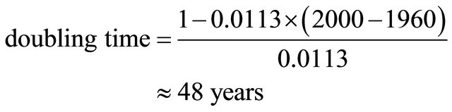
Similar calculations for the period ending in 1850, we get a doubling time of about 178 years, quite close to the actual doubling time in the range of 150 years. Also, for the period ending in 1600, we get a doubling time of about 450 years, again quite close to the 500 - 600 year doubling time observed during this epoch. Therefore, we see that the hyperbolic growth model has the nice feature of varying doubling times, mirroring real world data.
5. The Number of People Who Have Lived
We can do some very interesting things with the hyperbolic model, since it matches the past fairly well, such as answer the question, “How many people have lived on earth since the birth of Jesus?”
If we look at the model’s equation,
 which describes the curve of population growth over time, we see that we can integrate this equation between two time points:

to get the total person-years between time t1 and time t2.
We can integrate by substitution, letting and so
 , and we have
 , which simplifies to
 .
.
Recalling that we calculated P0 and k with t = 1960 as the baseline t0, and that the current year, which we designate as t2, is 2012, we can now rewrite this as:
Finally, plugging in  we have our final form, and we can calculate the number of person-years that have elapsed since the year 1 AD, by letting t1 = 1. Doing the calculation, we get about 1083 billion person-years.
To get how many people have lived since the year 1AD, we need to divide this number by the average life expectancy of people over this era. This is a very difficult estimate. Population expert Carl Haub states in a recent article that “life expectancy at birth averaged only about 10 years for most of human history” [5]. This was contributed to by a very high infant mortality rate during much of human history. Trying to account for the more recent increases in life expectancy, we’ll use an average value of 20 years. Doing this, we get 1083 billion person-years/20 years, or about 54 billion people. Thus, of all the people who have lived since the year 1 AD, more than 1 out of 8 is alive today.
Now, we want to answer the question posed by Carl Haub, “How Many People Have Ever Lived on Earth?”
Since homosapiens have existed since about 100,0000 BC, we can set  in our equation:

Doing that gives us a value of about 2134 billion person-years. Again, using an average life span over the length of human history of 20 years, we get that about 107 billion humans have lived on the earth since the dawn of history. This is extremely close to the current estimates of 108 billion [6].
6. Conclusion
Mathematical modeling of population growth provides an excellent tool both to predict and forecast future population growth, as well as to answer questions about the past. In this paper, we explored the exponential growth model, and used it to forecast the future. While there was an excellent fit to the data from the 1900’s, the exponential growth model did not show a good fit to more distant population data. Therefore, we developed a hyperbolic growth model, which showed excellent data fits with the past, but is clearly flawed in predicting the future. Therefore, one has to always test models against real data, and to carefully know the strengths and weaknesses of each model. Also, it is important to note that accurate predictions of population growth are much more complicated than the simple models presented above. Such predictions must take into account such factors as the age distribution of the population, birth rates, death rates, and scarcity of resources as a population grows. The interested reader is referred to fuller treatments of these issues in the works of Pollard [7] and Song and Jingyuan [8].
REFERENCES
- R. B. Banks, “Slicing Pizzas, Racing Turtles, and Further Adventures in Applied Mathematics,” Princeton University Press, Princeton, 1999, pp. 138-145.
- The United States Census Bureau, “Atlas of World Population History”. http://www.census.gov/population/international/data/worldpop/table_history.php
- Google Public Data. http://www.google.com/publicdata/explore?ds=d5bncppjof8f9_&met_y=sp_pop_totl&tdim=true&dl=en&hl=en&q=world+population+data
- Hyperbolic Growth. http://en.wikipedia.org/wiki/Hyperbolic_growth
- “How Many People Have Ever Lived on Earth?” Population Today: News, Numbers and Analysis, NovemberDecember 2002, Vol. 30, No. 8. http://www.prb.org/pdf/PT_novdec02.pdf
- “With Earth’s Population Now at 7 Billion, How Many People Have Ever Lived,” Nancy Szokan, Washington Post, October 31, 2011. http://www.washingtonpost.com/national/health-science/with-earths-population-now-at-7-billion-how-many-people-have-ever-lived/2011/10/27/gIQA6SLtZM_story.html
- A. H. Pollard, “Mathematical Models for the Growth of Human Populations,” Cambridge University Press, Cambridge, 1973.
- J. Y. Song, “Population System Control,” Mathematical and Computer Modeling, Vol. 11, Springer-Verlag Publishing, Berlin, 1988, pp. 11-16.