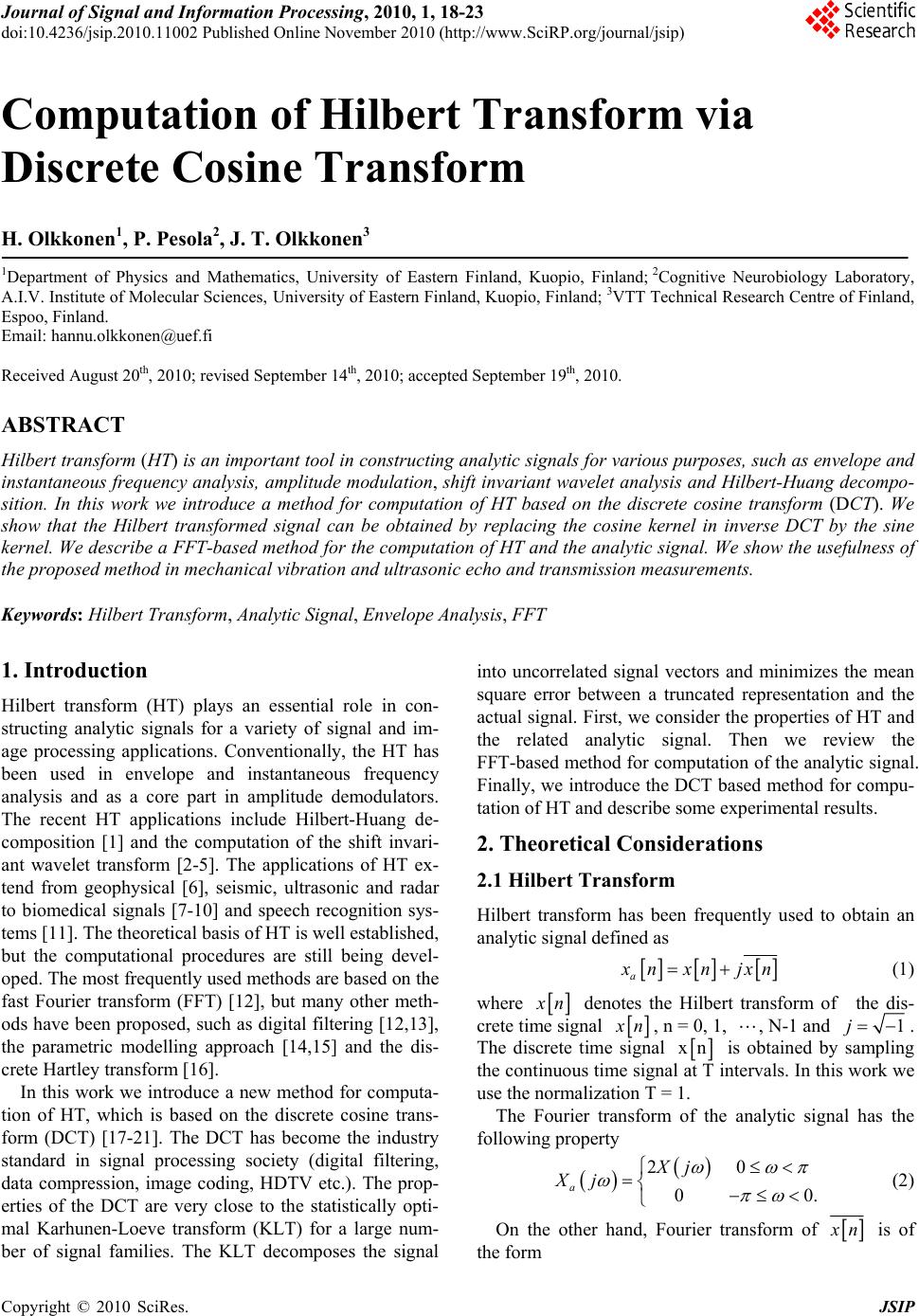Journal of Signal and Information Processing, 20 10 , 1, 18 -23
doi:10.4236/jsip.2010.11002 Published Online November 2010 (http://www.SciRP.org/journal/jsip)
Computation of Hilbert Transform via
Discrete Cosine Transform
H. Olkkonen1, P. Pesola2, J. T. Olkkonen3
1Department of Physics and Mathematics, University of Eastern Finland, Kuopio, Finland; 2Cognitive Neurobiology Laboratory,
A.I.V. Institute of Molecular Sciences, University of Eastern Finland, Kuopio, Finland; 3VTT Technical Research Centre of Finland,
Espoo, Finland.
Received August 20th, 2010; revised September 14th, 2010; accepted September 19th, 2010.
ABSTRACT
Hilbert transform (HT) is an important tool in constructing analytic signals for various purposes, such as envelope and
instantaneous frequency analysis, amplitude modulation, shift invariant wavelet analysis and Hilbert-Huang decompo-
sition. In this work we introduce a method for computation of HT based on the discrete cosine transform (DCT). We
show that the Hilbert transformed signal can be obtained by replacing the cosine kernel in inverse DCT by the sine
kernel. We describe a FFT-based method for the computation of HT and the analytic signal. We show the usefulness of
the proposed method in mech anical vibration and ultrasonic echo and transmission measuremen ts.
Keywords: Hilbert Transform, Analytic Signal, Envelope Analysis, FFT
1. Introduction
Hilbert transform (HT) plays an essential role in con-
structing analytic signals for a variety of signal and im-
age processing applications. Conventionally, the HT has
been used in envelope and instantaneous frequency
analysis and as a core part in amplitude demodulators.
The recent HT applications include Hilbert-Huang de-
composition [1] and the computation of the shift invari-
ant wavelet transform [2-5]. The applications of HT ex-
tend from geophysical [6], seismic, ultrasonic and radar
to biomedical signals [7-10] and speech recognition sys-
tems [11]. The theoretical basis of HT is well established,
but the computational procedures are still being devel-
oped. The most frequently used methods are based on the
fast Fourier transform (FFT) [12], but many other meth-
ods have been proposed, su ch as digital filtering [12,13],
the parametric modelling approach [14,15] and the dis-
crete Hartley transform [16].
In this work we introduce a new method for computa-
tion of HT, which is based on the discrete cosine trans-
form (DCT) [17-21]. The DCT has become the industry
standard in signal processing society (digital filtering,
data compression, image coding, HDTV etc.). The prop-
erties of the DCT are very close to the statistically opti-
mal Karhunen-Loeve transform (KLT) for a large num-
ber of signal families. The KLT decomposes the signal
into uncorrelated signal vectors and minimizes the mean
square error between a truncated representation and the
actual signal. First, we consider th e properties of HT and
the related analytic signal. Then we review the
FFT-based method for computation of the analytic signal.
Finally, we introduce the DCT based method for compu-
tation of HT and describe some experimental results.
2. Theoretical Considerations
2.1 Hilbert Transform
Hilbert transform has been frequently used to obtain an
analytic signal defined as






a
x
nxnjxn (1)
where


x
n denotes the Hilbert transform of the dis-
crete time signal


x
n, n = 0, 1, , N-1 and 1j

.
The discrete time signal


xn is obtained by sampling
the continuou s time signal at T intervals. In this work we
use the normalization T = 1.
The Fourier transform of the analytic signal has the
following property



20
00.
a
Xj
Xj




 
 (2)
On the other hand, Fourier transform of

x
n is of
the form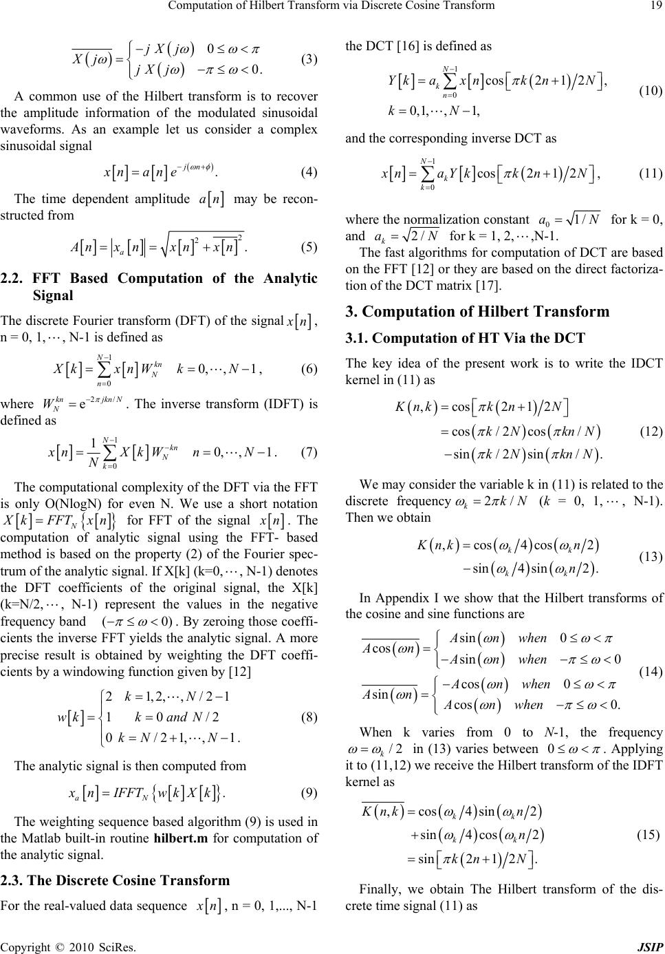

Computation of Hilbert Transform via Discrete Cosine Transform
19




0
0.
jX j
Xj jX j



 

 

 (3)
A common use of the Hilbert transform is to recover
the amplitude information of the modulated sinusoidal
waveforms. As an example let us consider a complex
sinusoidal sig n a l
 

.
jn
xn ane

 
 (4)
The time dependent amplitude


an may be recon-
structed from

2
2.
a
A
nxn xnxn  (5)
2.2. FFT Based Computation of the Analytic
Signal
The discrete Fourier transform (DFT) of the signal


x
n,
n = 0, 1,, N-1 is defined as
 
1
0
0, ,1,
Nkn
N
n
XkxnW kN



 (6)
where 2/
e
knjkn N
N
W
 
. The inverse transform (IDFT) is
defined as
 
1
0
10, ,1.
Nkn
N
k
xnXkW nN
N



 (7)
The computational complexity of the DFT via the FFT
is only O(NlogN) for even N. We use a short notation





N
X
kFFTxn for FFT of the signal


x
n. The
computation of analytic signal using the FFT- based
method is based on the property (2) of the Fourier spec-
trum of the analytic signal. If X[k] (k=0,, N-1) denotes
the DFT coefficients of the original signal, the X[k]
(k=N/2,, N-1) represent the values in the negative
frequency band (0)

  . By zeroing those coeffi-
cients the inverse FFT yields the analytic signal. A more
precise result is obtained by weighting the DFT coeffi-
cients by a windowing function given by [12]

21,2,,/21
10/2
0/21,,1.
kN
wkk andN
kN N





 



(8)
The analytic signal is then computed from







.
aN
x
nIFFTwkXk (9)
The weighting sequence based algorithm (9) is used in
the Matlab built-in routine hilbert.m for computation of
the analytic signal.
2.3. The Discrete Cosine Transform
For the real-valued data sequence


x
n, n = 0, 1,..., N-1
the DCT [16] is defined as
 

1
0
cos21 2,
0,1,,1,
N
kn
Ykaxnk nN
kN



 




(10)
and the corresponding inverse DCT as
 

1
0cos21 2,
N
k
k
x
naYk knN 







 (11)
where th e normalization constant 01/aN for k = 0,
and 2/
k
aN for k = 1, 2,,N-1.
The fast algorithms for computation of DCT are based
on the FFT [12] or they are based on the direct factoriza-
tion of the DCT matrix [17].
3. Computation of Hilbert Transform
3.1. Computation of HT Via the DCT
The key idea of the present work is to write the IDCT
kernel in (11) as






,cos 212
cos/ 2cos/
sin/ 2sin/.
Knkk nN
kN knN
kN knN



 



(12)
We may consider the variable k in (11) is related to the
discrete frequency2/
kkN



(k = 0, 1,, N-1).
Then we o bt a in





,cos4cos 2
sin4sin2.
kk
kk
Knk n
n



 (13)
In Appendix I we show that the Hilbert transforms of
the cosine and sine functions are




 

sin 0
cos sin 0
cos 0
sin cos 0.
Anwhen
AnAnwhen
Anwhen
AnAnwhen










 


 

 


(14)
When k varies from 0 to N-1, the frequency
/2
k



in (13) varies between 0

 . Applying
it to (11,12) we receive the Hilbert transform of the IDFT
kernel as
 


,cos4sin2
sin4 cos2
sin21 2.
kk
kk
Knkn
n
kn N










(15)
Finally, we obtain The Hilbert transform of the dis-
crete time signal (11) as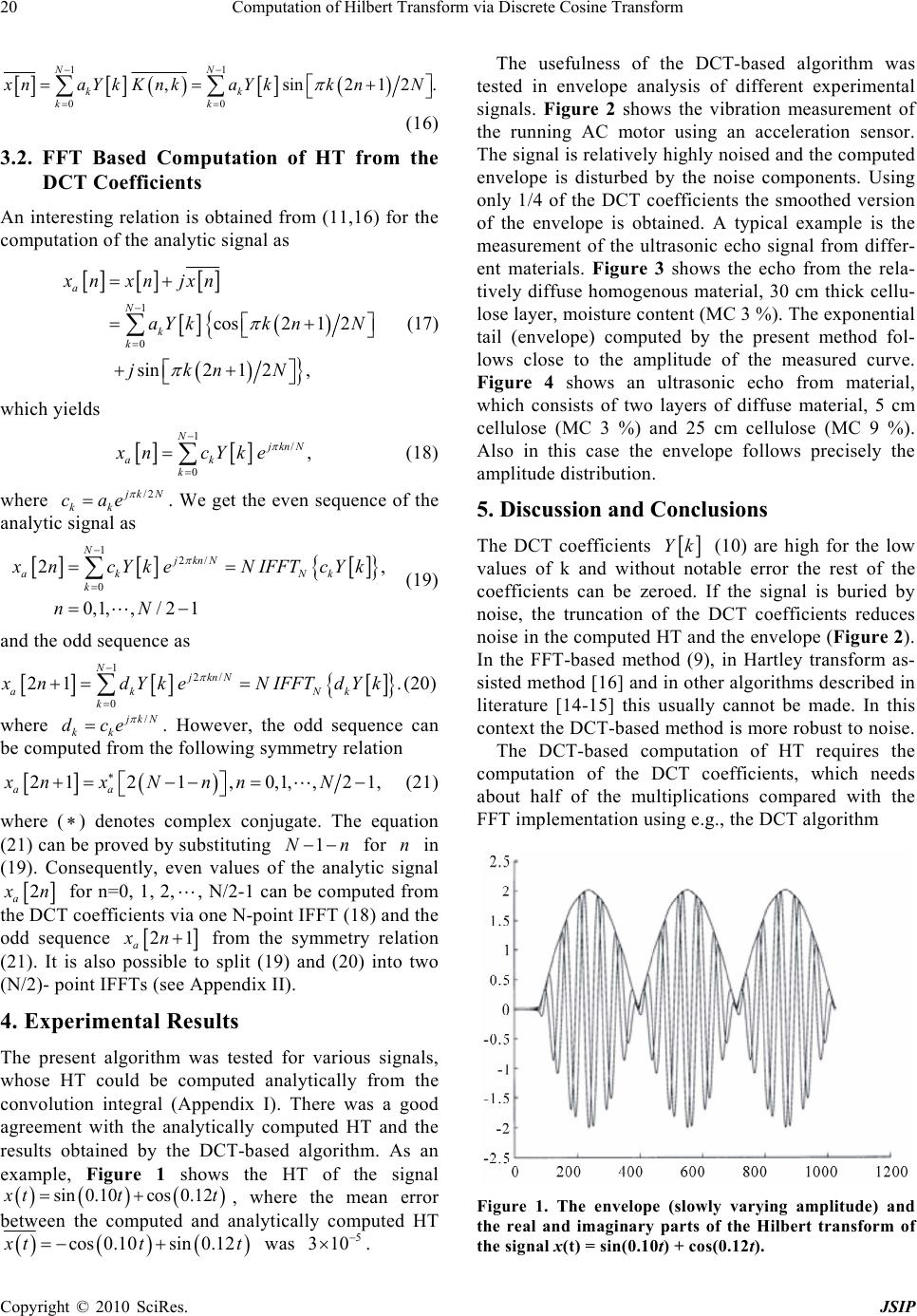

Computation of Hilbert Transform via Discrete Cosine Transform
20
 



11
00
,sin212.
NN
kk
kk
x
naYkKnkaYkk nN 


 


(16)
3.2. FFT Based Computation of HT from the
DCT Co effici ent s
An interesting relation is obtained from (11,16) for the
computation of the analytic signal as
 
 



1
0
cos21 2
sin21 2,
a
N
k
k
xn xnjxn
aY kknN
jknN












 (17)
which yields
 
1/
0,
N
j
kn N
ak
k
xn cYke



 (18)
where /2
j
kN
kk
cae

. We get the even sequence of the
analytic signal as
 

12/
0
2,
0,1,,/21
NjknN
ak Nk
k
xn cYkeNIFFTcYk
nN







(19)
and the odd sequence as
  
12/
0
21 .
NjknN
ak Nk
k
x
ndYkeNIFFTdYk



 
(20)
where /
j
kN
kk
dce

. However, the odd sequence can
be computed from the following symmetry relation



2121, 0,1,,21,
aa
xnx NnnN

 

 (21)
where () denotes complex conjugate. The equation
(21) can be proved by substituting 1Nn for n in
(19). Consequently, even values of the analytic signal


2
a
x
n for n=0, 1, 2,, N/2-1 can be computed from
the DCT coefficients via one N-point IFFT (18) and the
odd sequence


21
a
xn from the symmetry relation
(21). It is also possible to split (19) and (20) into two
(N/2)- point IFFTs (see Appendix II).
4. Experimental Results
The present algorithm was tested for various signals,
whose HT could be computed analytically from the
convolution integral (Appendix I). There was a good
agreement with the analytically computed HT and the
results obtained by the DCT-based algorithm. As an
example, Figure 1 shows the HT of the signal






sin 0.10cos 0.12
x
ttt , where the mean error
between the computed and analytically computed HT
 
cos 0.10sin 0.12
x
ttt  was 5 310

.
The usefulness of the DCT-based algorithm was
tested in envelope analysis of different experimental
signals. Figure 2 shows the vibration measurement of
the running AC motor using an acceleration sensor.
The signal is relatively highly noised and the computed
envelope is disturbed by the noise components. Using
only 1/4 of the DCT coefficients the smoothed version
of the envelope is obtained. A typical example is the
measurement of the ultrasonic echo signal from differ-
ent materials. Figure 3 shows the echo from the rela-
tively diffuse homogenous material, 30 cm thick cellu-
lose layer, moisture content (MC 3 %). The exponential
tail (envelope) computed by the present method fol-
lows close to the amplitude of the measured curve.
Figure 4 shows an ultrasonic echo from material,
which consists of two layers of diffuse material, 5 cm
cellulose (MC 3 %) and 25 cm cellulose (MC 9 %).
Also in this case the envelope follows precisely the
amplitude distribution.
5. Discussion and Conclusions
The DCT coefficients


Yk (10) are high for the low
values of k and without notable error the rest of the
coefficients can be zeroed. If the signal is buried by
noise, the truncation of the DCT coefficients reduces
noise in the computed HT and the envelope (Figure 2).
In the FFT-based method (9), in Hartley transform as-
sisted method [16] and in other algorithms described in
literature [14-15] this usually cannot be made. In this
context the DCT-based method is more robust to noise.
The DCT-based computation of HT requires the
computation of the DCT coefficients, which needs
about half of the multiplications compared with the
FFT implementation using e.g., the DCT algorithm
Figure 1. The envelope (slowly varying amplitude) and
the real and imaginary parts of the Hilbert transform of
the signal x(t) = sin(0.10t) + cos(0.12t).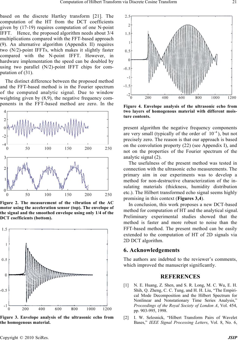

Computation of Hilbert Transform via Discrete Cosine Transform
21
based on the discrete Hartley transform [21]. The
computation of the HT from the DCT coefficients
given by (17-19) requires computation of one N-point
IFFT. Hence, the proposed algorithm needs about 3/4
multiplications compared with the FFT-based approach
(9). An alternative algorithm (Appendix II) requires
two (N/2)-point IFFTs, which makes it slightly faster
compared with the N-point IFFT. However, in
hardware implementation the speed can be doubled by
using two parallel (N/2)-point IFFT chips for com-
putation of (31).
The distinct difference between the proposed method
and the FFT-based method is in the Fourier spectrum
of the computed analytic signal. Due to window
weighting given by (8,9), the negative frequency com-
ponents in the FFT-based method are zero. In the
Figure 2. The measurement of the vibration of the AC
motor using the acceleration sensor (top). The envelope of
the signal and the smoothed envelope using only 1/4 of the
DCT coefficients (bottom).
Figure 3. Envelope analysis of the ultrasonic echo from
the homogenous material.
Figure 4. Envelope analysis of the ultrasonic echo from
two layers of homogenous material with different mois-
ture contents.
present algorithm the negative frequency components
are very small (typically of the order of 4
10

), but not
precisely zero. The reason is that our approach is based
on the convolution property (22) (see Appendix I), and
not on the properties of the Fourier spectrum of the
analytic signal (2).
The usefulness of the present method was tested in
connection with the ultrasonic echo measurements. The
primary aim in our experiments was to develop a
method for non-destructive characterization of the in-
sulating materials (thickness, humidity distribution
etc.). The Hilbert transformed echo signal seems highly
promising in this context (Figures 3,4).
In conclusion, this work proposes a new DCT-based
method for computation of HT and the analytical signal.
Preliminary experimental studies showed that the
method is faster and more robust to noise than the
FFT-based method. The present method can be easily
extended to the computation of HT of 2D signals via
2D DCT algorithm.
6. Acknowledgements
The authors are indebted to the reviewer’s comments,
which improved the manuscript significantly.
REFERENCES
[1] N. E. Huang, Z. Shen, and S. R. Long, M. C. Wu, E. H.
Shih, Q. Zheng, C. C. Tung, and H. H. Liu, “The Empiri-
cal Mode Decomposition and the Hilbert Spectrum for
Nonlinear and Nonstationary Time Series Analysis,”
Proceedings of the Royal Society of London A, Vol. 454,
pp. 903-995, 1998.
[2] I. W. Selesnick, “Hilbert Transform Pairs of Wavelet
Bases,” IEEE Signal Processing Letters, Vol. 8, No. 6,

Computation of Hilbert Transform via Discrete Cosine Transform
22
June 2001, pp. 170-173.
[3] H. Ozkaramanli and R. Yu, “On the Phase Condition and
Its Solution for Hilbert Transform Pairs of Wavelet
Bases,” IEEE Transactions on Signal Processing, Vol. 51,
No. 12, December 2003, pp. 3293-3294.
[4] R. Yu and H. Ozkaramanli, “Hilbert Transform Pairs of
Biorthogonal Wavelet Bases,” IEEE Transactions on
Signal Processing, Vol. 54, No. 6, part 1, June 2006, pp.
2119-2125.
[5] H. Olkkonen, J. T. Olkkonen and P. Pesola, “FFT Based
Computation of Shift Invariant Analytic Wavelet Trans-
form,” IEEE Signal Processing Letters, Vol. 14, No. 3,
March 2007, pp. 177-180.
[6] W. M. Moon, A. Ushah and B. Bruce, “Application of
2-D Hilbert Transform in Geophysical Imaging with Po-
tential Field Data,” IEEE Transactions on Geoscience
and Remote Sensing, Vol. 26, No. 5, September 1988, pp.
502-510.
[7] H. Olkkonen, P. Pesola, J. T. Olkkonen and H. Zhou,
“Hilbert Transform Assisted Complex Wavelet Trans-
form for Neuroelectric Signal Analysis,” Journal of Neu-
roscience Methods, Vol. 151, No. 2, pp. 106-113, 2006.
[8] H. Kanai, Y. Koiwa and J. Zhang, “Real-Time Measure-
ments of Local Myocardium Motion and Arterial Wall
Thickening,” IEEE Transactions on Ultrasonics, Ferro-
electrics, and Frequency Control, Vol. 46, No. 5, Sep-
tember 1999, pp. 1229-1241.
[9] S. M. Shors, A. V. Sahakian, H. J. Sih and S. Swiryn, “A
Method for Determining High-Resolution Activation
Time Delays in Unipolar Cardiac Mapping,” IEEE Tran-
sactions on Biomedical Engineering, Vol. 43, No. 12, De-
cember 1996, pp. 1192-1196.
[10] A. K. Barros and N. Ohnishi, “Heart Instantaneous Fre-
quency (HIF): An Alternative Approach to Extract Heart
Rate Variability,” IEEE Transactions on Biomedical En-
gineering, Vol. 48, No. 8, August 2001, pp. 850-855.
[11] O. W. Kwon and T. W. Lee, “Phoneme Recognition Us-
ing ICA-Based Feature Extraction and Transformation,”
Signal Processing, Vol. 84, No. 6, 2004, pp. 1005-1019.
[12] A. V. Oppenheim and R. W. Schafer, “Discrete-Time
Signal Processing,” Prentice-Hall, Englewood Cliffs,
1989.
[13] K. L. Peacock, “Kaiser-Bessel Weighting of the Hilbert
Transform High-Cut Filter,” IEEE Transactions on Aco us-
tics, Speech, and Signal Analysis, Vol. 33, No. 1, Febru-
ary 1985, pp. 329-331.
[14] A. Rao and R. Kumaresan, “A Parametric Modeling Ap-
proach to Hilbert Transformation,” IEEE Signal Process-
ing Letters, Vol. 5, No. 1, January 1998, pp. 15-17.
[15] R. Kumaresan, “An Inverse Signal Approach to Com-
puting the Envelope of a Real Valued Signal,” IEEE Sig-
nal Processing Letters, Vol. 5, No. 10, October 1998, pp.
256-259.
[16] S. C. Pei and S. B. Jaw, “Computation of Discrete Hilbert
Transform through Fast Hartley Transform,” IEEE Tran-
sactions on Circuits and Systems, Vol. 36, No. 9, 1989,
pp. 1251-1252.
[17] N. Ahmed, T. Natajaran and K. R. Rao, “Discrete Cosine
Transform,” IEEE Transactions on Computers, Vol. 23,
1974, pp. 90-94.
[18] C. W. Kok, “Fast Algorithm for Computing Discrete
Cosine Transform,” IEEE Transactions on Signal Proc-
essing, Vol. 45, No. 3, March 1997, pp. 757-760.
[19] G. Bi and L. W. Yu, “DCT Algorithms for Composite
Sequence Lengths,” IEEE Transactions on Signal Proc-
essing, Vol. 46, No. 3, March 1998, pp. 554-562.
[20] V. Britanak, P. Yip and K. R. Rao, Discrete Cosine and
Sine Transforms: General Properties, Fast Algorithms and
Integer Approximations, Academic Press Inc., Elsevier
Science, Amsterdam, 2007
[21] H. Malvar, “Fast Computation of the Discrete Cosine
Transform and the Discrete Hartley Transform,” IEEE
Transactions on Acoustics, Speech, Signal Processing,
Vol. 35, No. 10, October 1987, pp. 1484-1485.

Computation of Hilbert Transform via Discrete Cosine Transform
23
Appendices
1. Hilbert Transform of the Cosine Function
The Hilbert transform of the continuous time signal x(t)
can be defined b y the convolution as
  
11 ,0,1,,1.
x
xtxtd nN
tn




 

 (22)
For the discrete time signal x[n] we may write

 1,0,1,,1.
xt
xndtnN
nt





 (23)
Now we may calculate the Hilbert transform of



cos
x
nA n  
  

cos
cos
cos .
nt
t
AA
A
ndtdt
nt t




 




(24)
The last result is due to the general property of the
convolution integral


 
.
x
tydxytd

  

(25)
By expanding


 


coscos cossin sinntntnt

    we
obtain
 




cos sin
cos cossin.
tt
AA
A
nndtndt
tt

 


 


(26)
Since we have
 
cos sin
0,
tt
dt dt
tt



 


(27)
we obtain the final result
 

sin 0
cos sin 0.
Anwhen
AnAnwhen







 (28)
In a similar manner we may prove



cos 0
sin( )cos 0.
Anwhen
An
Anwhen






 

 (29)
2. Alternative Computational Method for (17)
and (18)
We may split (17) into two parts
 



21
122
22
00
22
2
21
22
21 ,
N
NjknN
jknN
ak k
kk
jknN
jnN
k
xn cYkecYke
cYk ee











(30)
which gives the even values
  
 
22
2221
22
2
21.
2
aNk
jnN Nk
N
xnIFFTcYk
N
eIFFTcYk




(31)
Correspondingly, the odd values are obtained from
 

 
22
2221
21 2
2
21.
2
aNk
jnN Nk
N
xnIFFTd Yk
N
eIFFTdYk


 

(32)
If we denote the even values in (28) as






12
2,
a
x
nxnxn (33)
then the odd values are obtained from






12
21/21/21 .
a
x
nxN nxN n

 (34)
The result (34) can be proved by direct substitution of
/2 1Nn

for n in (30).