Advances in Materials Physics and Chemistry
Vol.06 No.07(2016), Article ID:67958,18 pages
10.4236/ampc.2016.67019
Examples of Non-Uniqueness of the Equilibrium States for a Floating Ball
Ray Treinen
Department of Mathematics, Texas State University, San Marcos, Texas, USA

Copyright © 2016 by author and Scientific Research Publishing Inc.
This work is licensed under the Creative Commons Attribution International License (CC BY).
http://creativecommons.org/licenses/by/4.0/


Received 26 April 2016; accepted 2 July 2016; published 5 July 2016
ABSTRACT
We provide a numerical algorithm for numerically approximating a centrally located floating ball. We give examples of equilibria, and we present non-unique cases for the same physical parameters when the density of the ball is either greater than the supporting liquid (heavy) or lighter than the density of the vapor above (light). We classify the non-uniqueness by analyzing a function related to the force balance. We derive the potential energy of these states, and make comparisons of the non-unique cases. In the cases of both the light and heavy floating balls, the evidence presented supports the conjecture that when there are two equilibria, the one with lower energy corresponds to the location of triple junction (between the ball, the vapor and the liquid) that is closer to the equator of the ball.
Keywords:
Floating Ball, Capillarity

1. Introduction
Consider a ball of density  floating at the surface of a fluid that has density
 . We present numerical examples of non-uniqueness of the equilibrium states for these configurations. We will also provide a framework for the classification of these states, including an energy analysis. The energy analysis is used to determine which of the two equilibria has the lower energy, and thus, at least amongst centrally located floating balls, this process finds the energy minimizing configuration. Under these conditions, this is the configuration that our model predicts which will be found in experiments. We begin with a precise formulation of our model.
The energies considered in this model are due to the surface tension and gravity. Surface tension energy is taken, as usual, to be proportional to the area of the free surface with proportionality constant  called the surface tension constant. The energy due to gravity consists of two terms, one corresponding to the liquid and another to the floating object. The former is proportional to the density of the liquid,
  , a gravitational constant, and a volume integral of the physical height, z, in the gravity field. The latter is similar except the density of the floating object,
  , is used, and the integral is taken over the volume of the floating object. If we denote the floating ball by B, the liquid by E, and
  the free liquid-air interface,
  the wetted portion of the bounding walls, if they exist,
  the wetted portion of the floating ball. Then the energy of this configuration is given by
 (1)
(1)
with wetting coefficients  and
and , depending on contact angles
  and
and  at the contact with the ball and the wall, respectively. Here z is height in the vertical direction, and
  is the volume measure. Also,
  denotes surface area, calculated using a Hausdorff measure, as appropriate. It is often convenient to refer to the mathematical energy of the system, which is merely the scaled energy
 . Note that then the gravitational terms become

with “capillary constant” .
.
The natural physical setting for these problems is in a bounded container in . We will study the lower dimensional problem here for two reasons: first, there is a growing literature of flotation in this setting, and second, there is an approach to prove the existence (and, when applicable, uniqueness) of the equilibria in this setting using a phase plane analysis; and it is useful to have robust numerical simulations. We will consider the settings in
  of both a bounded container and an unbounded sea of fluid. We can interpret these problems as the lower dimensional setting, or we can interpret them as unbounded in one horizontal direction. In the latter, the floating ball may be seen as an infinitely long log floating in an infinitely long trough. The triple contact line of the liquid with the air at the surface of the floating object is then a straight line extending along the unbounded log. In what follows we preserve the intuitive meaning of area, volume, and energy by interpreting the lower dimensional setting as generating cylindrical configurations in the unbounded horizontal direction, and then we take the area, volume, and energy to be per unit distance in that unbounded direction.
The goal of this note is to provide numerically computed approximations to some sample configurations when the ball is centrally located in the container and the fluid is assumed to be symmetric about the central axis. We will focus on the cases of the density  outside of the range
 . One could classify the admissible densities into three types: light, medium, and heavy. This would correspond to
 ,
,  , and
, and , respectively. Specifically, we will classify the behavior of a certain function
  that is pivotal in the force balance considerations, as derived using variational techniques. Then we will follow this by a measurement of the mathematical energy, specifically of interest for the cases of non-uniqueness. For a theoretical treatment of this setting in general, see first McCuan and Treinen [1] , and also McCuan [2] for further details. We will use the results of those variational arguments in what follows.
With this setting established, we are able to proceed to the configurations of interest. Assume that the ball floats centrally, and so that the center of the ball is at a height d. Thus the boundary of the ball can be described by its azimuthal angle  and its radius a, given a height d. The fluid-air interface contacts the ball at a particular azimuthal angle, denoted by
 . In the bounded cases a volume of fluid is described by the wetted container walls, the fluid-air interface, and the wetted surface of the ball. This volume is held fixed, and introduces a Lagrange multiplier
  into the problem. The height of the fluid is given by the differential equation

where  is the mean curvature operator, commonly seen as

where

when the surface is a graph over some base domain. However, we will not restrict ourselves to these limited configurations. We have boundary conditions

where  is the exterior unit normal on the container, or the interior unit normal on the ball, as appropriate. Also,
  is taken to be the contact angle along the container wall, or the ball itself, also we assume that
  is constant, up to possibly having different values on the container wall and on the ball, as described above. This restriction that
  is locally a constant is simply a statement that we are considering only uniform materials in this current work. The underlying model is flexible enough to accommodate non-constant
 , if
, if  is well behaved.
In [1] , we derived an additional necessary condition that does not appear in the classical literature consisting of fluid interactions with rigid solid objects. A manuscript by Finn [3] is the standard reference for the classical literature. We need to define several objects before we can state this condition. Denote the volume of fluid by . Set
. Set  to be the outward pointing unit co-normal along the boundary of the liquid-air interface. Set N to be the unit normal to
  pointing out of
 . The fluid-air interface has a surface tension
 , and the potential
energy due to gravity is measured as  where G depends on position and the material. For our application, if z measures height in the vertical direction, then
 , for the appropriate density
 . Then the condition for free floating is
 (2)
(2)
Under the assumption of symmetry about the vertical axis, the PDE with boundary conditions can be reduced to
 (3)
(3)
This representation of the equation allows for the parameterized curve to pass through both inflection points and vertical points. Various authors have studied this system with differing boundary conditions and also as a family of solution curves. Solutions are sometimes known as Euler elastica. See Aspley, He, and McCuan [4] , Euler [5] , Giaquinta and Hildebrandt [6] (pp. 142-144), McCuan [7] and [8] , and Wente [9] for both historical origins, as well as applications to capillarity.
Then (2) becomes
 (4)
(4)
and we define  to be the left hand side of this equation. A key observation is that the locally observed information is collected on the left side of this equation, and the right side contains the global density information. In [1] we interpreted this as a version of a force balance condition.
We seek solutions to (3) that satisfy (4) and  where
where  is some prescribed quantity of volume large enough that the ball need not touch the container. This problem is the bounded container problem in
 . The unknown quantities are
 . The details are in Section 2.1.
If we replace the bounded container with an infinite sea of liquid, then we follow Bhatnagar and Finn [10] in taking the Lagrange multiplier  to be 0, and the condition
  when
when  is replaced with
 . We then seek solutions to (3) thus modified that satisfy (4) with
 . This problem is the unbounded container problem in
 . This problem is significantly simpler, and one may view it as adding assumptions compared to the bounded container problem, the result of which is a family of curves representing the fluid interface that is completely characterized. In fact, it can be shown that not only is there existence and uniqueness of the boundary value problem in this setting, but we also have a formula for both
  and
and . (See [10] , though unfortunately the formula is stated incorrectly there.) Thus the unknown quantities in the 2D unbounded container problem are reduced to
 . The details are in Section 2.2.
Before moving on to these details we would like to mention some other authors and their works on floating objects: Bemelmans, Galdi, Kyed [11] , Bhatnagar and Finn [10] , Finn [12] - [14] , Finn, McCuan, and Wente [15] , Finn and Sloss [16] , Finn and Vogel [17] , Kemp and Siegel [18] , McCuan [2] , Vella [19] , Vella and Mahadevan [20] , Vella, Lee, and Kim [21] , and Vella, Metcalfe, and Whittaker [22] . In particular, as pointed out in [19] , a number of applications have been of recent interest, for some examples, see capillary-driven self-assembly Whitesides and Boncheva [23] and Whitesides and Grzybowski [24] , the stabilization of emulsions by colloidal particles (Binks and Horozov [25] , Tavacoli, Katgert, Kim, Cates and Clegg [26] ), the locomotion of insects and spiders on water (Bush and Hu [27] , Gao and Jiang [28] ), and the design and optimization of biomimetic water-walking robots (Hu, Chan and Bush [29] , Ozcan, Wang, Taylor and Sitti [30] , Song and Sitti [31] ).
2. Methods
We will consider first the bounded container in , followed by the unbounded container. In both of these configurations there is a common method of approach. The floating ball problem is cast as solving a system of ODEs coupled with side conditions for the volume constraint and the new free boundary condition. The side conditions can be considered simultaneously with the standard boundary conditions, and form a set of necessary conditions. We employ shooting methods for the underlying systems of ODEs coupled with nonlinear zero finding algorithms for vectorized necessary conditions. The zero finding algorithms require initial guesses for the free parameters, which we tune to the given physical with estimates when we are able.
Next we illustrate how the new free boundary condition can be used to determine when there is non uni- queness of the equilibria. We give numerical examples. Finally, in the case of the bounded container, we calculate the potential energy of each configuration and compare the energy of the two configurations with the same physical properties.
2.1. Bounded Container in R2
We first need to measure the volume of fluid held in the container. One may compute
 (5)
(5)
Our formula does not require that the height u is a function over a base domain.
In what follows we will assign  in all of the numerical computations. This can be seen as applying a standard scaling argument, however we are then unable to further normalize the container described by R, and the radius of the ball a. Thus these two parameters are inherent features of this model.
The numerical procedure is a shooting method, where we integrate the system of ODEs
 (6)
(6)
with initial conditions
 (7)
(7)
to some ending arc-length  using ODE45 in Matlab. We use the finest permitted tolerances, with the absolute tolerance set to
  and the relative tolerance set to
 . We have free parameters
 , and
, and . We use these to satisfy the physical conditions
 (8)
(8)
 (9)
(9)
 (10)
(10)
 (11)
(11)
which say that the configuration satisfies the volume constraint and the force balance condition as well as the need for the fluid interface to extend to the wall of the container with the prescribed contact angle.
The parameters  are given the following initial guesses:


This leads to a solution of the initial value problem where we can evaluate the conditions (8)-(11). We use Matlab’s fsolve to then vary , computing the solution to the IVP out to the arc-length
  at each step, until Equations (8)-(11) are satisfied up to the requested tolerances. Matlab’s fsolve uses a dogleg variant of a trust region method to solve this 4-dimensional zero finding problem. Here we use tolerances that are coarser than the underlying ode solver’s tolerances, as the zero finding depends on those approximations. Specifically, we use termination tolerance on the objective function value of
  and on the input values of
 .
.
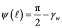
We next proceed with a few examples. In Figure 1 we set ,
,  ,
,  and
and , and compare
  values of 0 and
 . We conjecture that the figure on the left shows a stable configuration, while the figure on the right shows a configuration conjectured to be unstable. In order to analyze this stability criterion, we would need to consider off-center configurations, which we leave for a future work. In Figure 2 we set
  and
and , and compare
  with
with  values of 0.20058 on the left and 0.69924 on the right. We conjecture that the figure on the left shows a local energy minimum, and the figure on the right shows an energy maximum.
As an approach to explain the behavior in the examples in the second pair, we turn to a study of the function . The parameters
  are given the same initial guesses as just above, with an initial value of
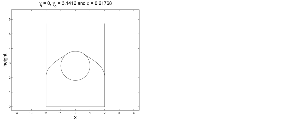

Figure 1. Comparing contact angles  set to
  on the left and 0 on the right.
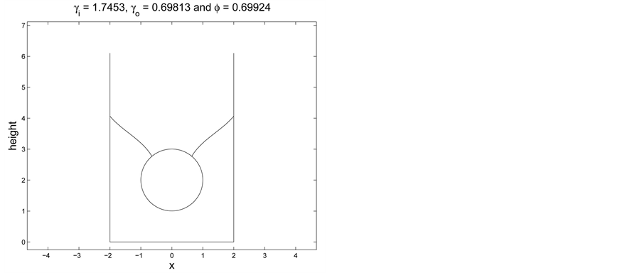

Figure 2. Non-uniqueness: two values of  for the same physical parameters.
 . This leads to a solution of the IVP which we can use to evaluate the following conditions to within a given tolerance:


and we use Matlab’s fsolve to then vary , computing the solution of the IVP out to the arc-length
  at each step, until the equations for the necessary conditions are satisfied up to a given tolerance. Then we evaluate
  with this information. We proceed iteratively for evenly spaced values of
  using the data from previous step as an initial guess for each new value of
 . The range
  is treated in the same manner.
We do not attempt to evaluate , nor
, nor , however, we use the limiting values of
  and
and . We sample from this process in Figure 3 and Figure 4. Notice that we have included the non physical immersed partial solution to the floating ball problem. We call these semi-equilibria.
We show the plot of F for  and
and  compared to
  and
and  in Figure 5. Take careful note of a key fact. In the
  example, there are apparently no solutions to the floating ball problem when
 , as
, as  here. We include some endpoints of the
  pairs: see Figure 6 with
  and
and .
.
With these solutions to the partial floating ball in hand, we are able to numerically calculate the energy of the configuration. It is simpler to use the scaled mathematical energy , and we also use the standard scaling arguments that result in
  and
and . The free interface energy
  is simply
 , and the wetting
energies are also trivial to compute:  and
and . We then calculate the gravita- tional potential energy of the ball:
 (12)
(12)
The gravitational potential energy of the liquid is more convenient to compute in sections. First we will treat the portion directly below the interface, but due to the lack of a closed form expression and also due to the variable step size of the data we do this numerically with the trapezoid rule:


Figure 3. Computing partial solutions for values of .
.
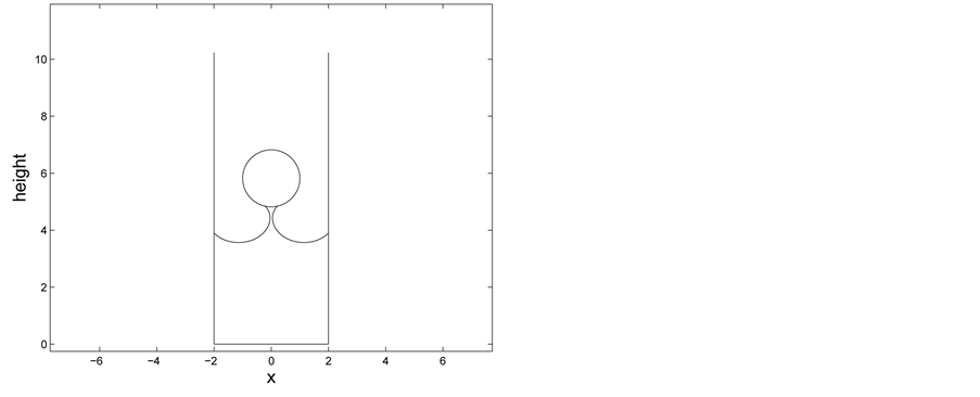
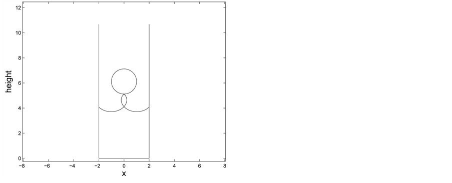
Figure 4. Computing partial solutions for values of .
.
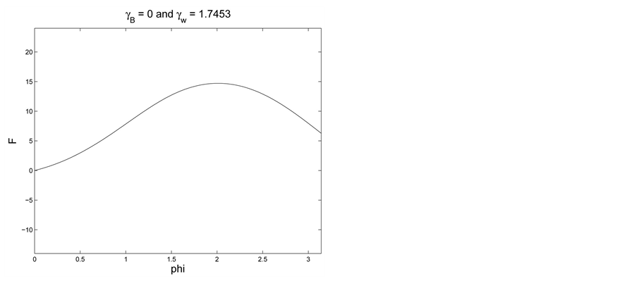
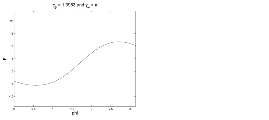
Figure 5. Symmetric values of contact angles.
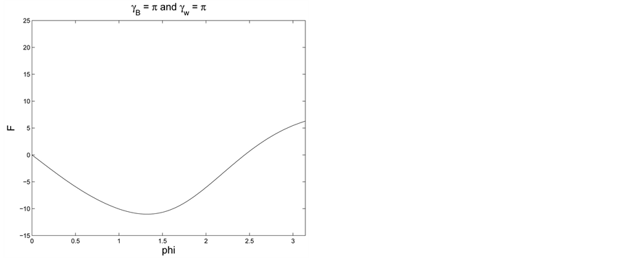
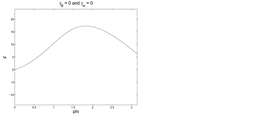
Figure 6. At the extreme range of  pairs.
where . The error here is bounded by
 (13)
(13)
where h is the maximum step size taken in the irregularly spaced data, and  is some number in the interval
 . If
. If , then we simply need to add to this quantity the portion directly under the ball that has not yet been accounted for:
 (14)
(14)
 (15)
(15)
The case where  has the complication that we must remove the portion of the fluid where the ball overlaps the portion directly below the free interface. We find the formulas match if we additionally compute the energy from the top of the ball, then subtract the entirety of the corresponding energy of the ball:
 (16)
(16)
 (17)
(17)
which matches (15) upon subtracting , the energy of the whole ball.
2.2. Unbounded Container in R2
We next consider the unbounded container problem in . This is envisioned as an infinitely long log floating on an unbounded sea of liquid. As such, there is only the contact angle on the ball, so we use
 . It is worth noting that the only relative relation remaining is that comparing a to
 . In the case of the bounded container there is the significantly more complicated interaction between a, R, and
 , as well as the contact angle
 . We are first interested in finding a solution to
 (18)
(18)
that satisfies  and
and . The curve
  forms a generating curve for the cylindrical liquid-air interface. This system is equivalent to the following system
 (19)
(19)
 (20)
(20)
satisfying  and
and . This can be explicitly integrated:
 (21)
(21)
 (22)
(22)
See [10] and [9] .
We proceed to the full problem of computing the floating ball configuration in the unbounded  configuration. Using our formulas, for each
  we can produce an interface curve
  that begins
with inclination angle  where
where . Then we set
  to fix the height of the ball. We are then able to evaluate the necessary condition
 (23)
(23)
with . We are left with this single equation as well as one free parameter:
 . We use Matlab's zero finding function FZERO to vary
 , computing the solution to the asymptotic boundary value problem at each step, until this equation is satisfied to within given tolerance.
Our results can be compared to Bhatnagar and Finn [10] , where an independent variational formulation was used. In our case, we are formally applying the results from [1] which assumed a bounded container in order to measure the energy of the configuration, whereas in [10] their variational argument was constructed with care to account for the difficulties of infinitesimal variations of infinite quantities.
Our examples use . In Figure 7 we show non-uniqueness with
 . The configuration on the left is conjectured to be stable, with a value of
 , and the configuration on the right is conjectured to be unstable, with a value of
 . In comparison, there was only one solution when
 : Figure 8.


Figure 7. Non-uniqueness: two values of  with
with .
.

Figure 8. Unique solution with the same contact angle and .
.
3. Results and Discussion
We begin here with the floating ball in a bounded container, and we ask the following question: what values of  pairs give non-uniqueness of one or both of
  and
and ? Proceeding as before, for
 , we compute F as above and then test the regions
  and
and  for monoto- nicity. The results appear in Figure 9 with Figure 10. It is worth mentioning that there are 50 grid points on each axis, and
  was evaluated at 100 grid points of
 , giving 250,000 numerical solutions to the (partial) floating ball problem for each of these figures. The cases marked with a star represent curves that begin at
 , and
, and , proceeding down to a global minimum, where
 . Then F increases to its global maximum, where
 , and then decreases to its terminal values at
 . Note
 . The cases marked with a square represent curves that begin at
 , and
, and , proceeding to its global maximum, from which it decreases to its terminal value at
  where
where . This gives non- uniqueness for
  only. The cases marked with a plus represent curves that begin at
 , and
, and , proceeding to its global minimum, from which it increases to its terminal value at
  where
where . Here non-uniqueness appears only for
  only.
only.
It should be stated that while this current work focuses more directly on the influence of the contact angles on the nonuniqueness criterion, the influence of R and a on the nonuniqueness criterion is just as important. To see this impact, compare Figure 9 with Figure 10. We leave a separate study focusing on fixed contact angles and varied values of R and a for a further work.
With the energy computed as in Section 2.1, we first use it in conjunction with the graph of . For each semi-equilibria with
  we compute the mathematical energy of that configuration. This curve is
plotted with that of  in Figure 11. Carefully note that the density of the ball changes along this curve. We do not specify a fixed density, however, we back out the density that appears in the graph of
  with the observation that

Then the energy is computed with this value of . Further, the energies of the two equilibria are compared in Figure 11, and at least for the particular height picked to illustrate this energy difference, the equilibria with

Figure 9. Non-uniqueness of equilibria for  and
and .
.

Figure 10. Non-uniqueness of equilibria for  and
and .
.

Figure 11. Using the function F to determine which solution has the lower energy. The curves are F and the energy. The lower horizontal line fixes a height that picks up two values of  for the same value of F (and thus
 ). These two
  values are indicated by the vertical lines. Finally, the upper horizontal line is shown that meets the intersection of the energy graph and the rightmost vertical line. Note that the energy is below the intersection of the upper horizontal line and the left vertical line. This implies the configuration with the smaller value of
  has lower energy.
the smaller value of  has lower energy. For a more robust comparison, consider first the light ball. If there is non-uniqueness, there is a maximum value of F with
  there. Denote this value by
 . Next, we pick the subset of the
  values in
  and for each of these, we use the value of
  to interpolate the smaller value of
  that shares the same height of F. Finally, we interpolate the energy at this smaller value of
 . Then we plot the energy for
  in
in  and the corresponding energy values that come from this comparison scheme. The results are shown in Figure 12. The corresponding comparison is done for the heavy floating ball, see Figure 13. In both of these cases the value of
  further away from the endpoints of the interval
  had lower energy than the other possibility. This is some evidence for the conjecture that the energy minimizer contacts the ball closer to the equator when compared to other equilibria. We will state this conjecture more precisely below.
We then included the above analysis into the program that generated Figure 9 with a 50 × 50 grid of values for  and
and , and the results are shown in Figure 14. A series of these simulations were performed amounting to 3.5 million tests of the conjecture. The results are in Table 1. The cases with
  and
and  were attempted, however the initial guess for the zero finding function needs to be refined in these cases, as those guesses had been tuned to configurations where the curvature was larger, and convergence to semi-equilibrium is not uniform on the grid considered. The cases
 ,
,  and
and  with
with  are at the limits of the ability to prescribe finer tolerances for the problem and the results are not conclusive for the cases we have considered there. We should note that in the case
 ,
,  we needed to prescribe the relative tolerance of Matlab’s ode45 to
  in order to verify the conjecture there. This became the standard for our tests, and as the spacing of floating point numbers is
 , we are currently unable to achieve finer results.
Next, we trace the energy values from a sampling of balls with given, fixed densities as the semi-equilibrium are computed through the range . This is in contrast to the energy graphs that we have so far

Figure 12. The light ball energy comparison.

Figure 13. The heavy ball energy comparison.
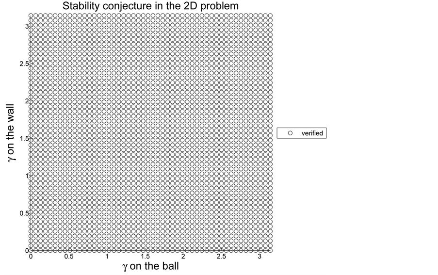
Figure 14. Verifying the conjecture with  and
and .
.

Table 1. The configurations where the conjecture was tested, with the displayed radius a and the half-container width R. Each entry on this table represents 250,000 configurations with 50 × 50 evenly spaced points of  pairs, and for each pair, 100 evenly spaced points were chosen for
 .
.
examined. Here we fix a few densities and in contrast, in the previous discussions the densities would vary with the value of . Figure 15 shows the results of this, which should be seen as following a ball as it rises from the depths, first registering when it contacts the interface with
  in a semi-equilibrium state, and passing continuously through that parameter until leaving the fluid at
 . It should be understood that this is not a continuous behavior in terms of the center height d. In fact, in order to achieve the semi-equilibria, in general d changes discontinuously at both the point of beginning and ending the contact with the free interface. We do not include that behavior in our graphs. The feature exhibited in these figures that that there are at most two interior local extrema along the trajectory of the energy profile curves. This is in agreement with the maximum of two equilibria for a fixed density, of either a light or heavy ball. The phenomenon can be described at follows, as the ball passes through a full range of heights, though not necessarily monotonically. First, let
 . Then, as d increases from the depths, the energy decreases. At the contact with the interface there will
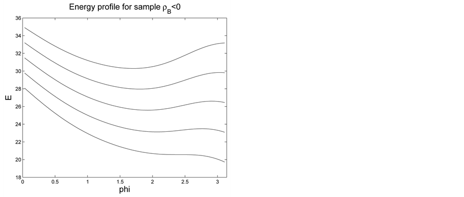

Figure 15. Given 5 sample densities , tracing the energy of the system as
  moves from 0 to
 . On the left
  and on the right
 .
.
be a discontinuous change in d. Then we move through the parameter , increasing from
  as the energy continues to decrease. Then there appears a local energy minimizer, where the surface energies play a stronger role than the gravitational energies. From this point the energy may increase from a local minimum, or decrease from a saddle point. On the remainder of the curve there may be a second equilibia, which is a local energy maximum. The energy is continuous to the endpoint where
 . At this point there is another discontinuous change in the height d as the ball frees itself from the interface, and from this point it continues upwards indefinitely as the energy continues to decrease. Second, let
 . Here the ball rises from the depths, with increasing energy up to the point of contact with the interface. Then there is a discontinuous change in d at the contact, but where the configuration is in a semi-equilibrium at
 . Then as
  increases, the energy decreases to a local energy minimizer. From there the energy increases, and there may be another equilibrium along the curve, which would be a local energy maximum. Either way, the energy is continuous up to the point where
 , and then there is another discontinuous change as the ball leaves the liquid. From there the ball continues upward, and the energy increases with d.
Finally, we turn to a study of  for the floating ball problem in an unbounded container. Adapting the argument from the case of an bounded fluid in
 , we generate F over
 . In this setting, however, once
 is removed from the list of unknowns, and
  is removed from the necessary conditions, we are able to generate a configuration for each
  using the explicit solutions as above.
Figure 16 shows the results for  and
and . Again, note the lack of a possibility of a solution existing if
  when
when . Also note that there is no solution possible if
  when
when . Figure 17 shows an example when it is possible to have non-unique solutions for both of the cases
  and
and  for that particular choice of
 .
.
We compute F over , testing the regions
  and
and  for monotonicity. The results are collected in Figure 18, where we display the results for a selection of radii
 . The behavior is in line with the simulations done with the bounded case in
 . We do not here proceed with an energy comparison between these non-unique cases for two reasons. First, the one approach that might be used would be to fix some large domain with which to measure the energies and compare the two values obtained. This is seemingly somewhat arbitrary, and has the possibility of not detecting the correct case when the comparison is close. Second, and more important, is that Bhagnagar and Finn [10] carefully analyzed the energy comparisons, and their method is superior to that just described. We do not wish to repeat their analysis, so we simply take note that their analysis supports the following conjecture in the examples that they computed explicitly. Further, Bhatnagar and Finn found examples of nonuniqueness, and their energy based methods give rise to a more

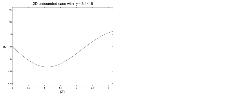
Figure 16.  with contact angles
 .
.
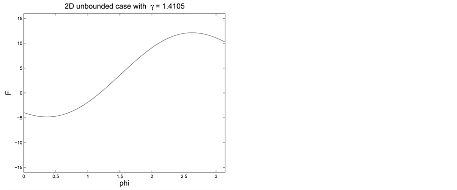
Figure 17. An example of  with nonuniqueness for both light and heavy floating balls.
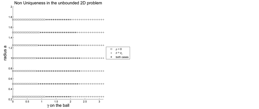
Figure 18. Nonuniqueness of equilibria with .
.
rigorous stability analysis. The results from this section then can be seen as purely an analysis of the non- uniqueness criteria.
Conjecture 1. The centrally located floating ball has at most two equilibria in a bounded container in 2D, and the centrally located floating ball has at most two equilibria in the unbounded configuration in 2D. In both cases, this will occur at some value or values of the azimuthal angle  on the ball. In the case that
 , if there are two configurations then the solution with the smaller value of
  has lower energy. In the case that
 , if there are two configurations then the solution with the larger value of
  has lower energy.
4. Conclusion
We have developed a robust numerical solver for finding the equilibria of a centrally located floating ball in both bounded and unbounded problems in . The non-unique cases for both the light ball and the heavy ball have been analyzed using the function
 , and the uniqueness and non-uniqueness depend on the geometry of the graph of that function. We calculated the potential energy of the bounded configurations, and used that first, to determine which non-unique equilibrium was the local energy minimizer, and second, to trace the energy profile of a ball as it is passed through the fluid interface. Our methods were used to formulate a conjecture on the energy minimizer, and 3.5 million test cases were verified.
Cite this paper
Ray Treinen, (2016) Examples of Non-Uniqueness of the Equilibrium States for a Floating Ball. Advances in Materials Physics and Chemistry,06,177-194. doi: 10.4236/ampc.2016.67019
References
- 1. McCuan, J. and Treinen, R. (2013) Capillarity and Archimedes’ Principle of Flotation. Pacific Journal of Mathematics, 265, 123-150.
http://dx.doi.org/10.2140/pjm.2013.265.123 - 2. McCuan, J. (2007) A Variational Formula for Floating Bodies. Pacific Journal of Mathematics, 231, 167-191.
http://dx.doi.org/10.2140/pjm.2007.231.167 - 3. Finn, R. (1986) Equilibrium Capillary Surfaces. Grundlehren der Mathematischen Wissenschaften [Fundamental Principles of Mathematical Sciences], Vol. 284, Springer-Verlag, New York.
http://dx.doi.org/10.1007/978-1-4613-8584-4 - 4. Aspley, A., He, C. and McCuan, J. (2015) Force Profiles for Parallel Plates Partially Immersed in a Liquid Bath. Journal of Mathematical Fluid Mechanics, 17, 87-102.
http://dx.doi.org/10.1007/s00021-014-0192-3 - 5. Euler, L. (1744) Methodus inveniendi lineas curvas maximi minimive pro-preitate gaudentes, sive solutio problematic isoperimetrici lattisimo sensu accpti. Ser. I, vol. 24, Bousquet, Lausannae et Genevae, E65A. O.O.
- 6. Giaquinta, M. and Hildebrandt, S. (1996) Calculus of Variations, I. Grundlehren der Mathematischen Wissenschaften [Fundamental Principles of Mathematical Sciences], Vol. 310, Springer-Verlag, Berlin.
- 7. McCuan, J. (2013) Extremities of Stability for Pendant Drops, Geometric Analysis, Mathematical Relativity, and Nonlinear Partial Differential Equations. Contemporary Mathematics, 599, 157-173.
http://dx.doi.org/10.1090/conm/599/11944 - 8. Mccuan, J. (2015) New Geometric Estimates for Euler Elastica. JEPE, 1, 387-402.
- 9. Wente, H.C. (2006) New Exotic Containers. Pacific Journal of Mathematics, 224, 379-398.
http://dx.doi.org/10.2140/pjm.2006.224.379 - 10. Bhatnagar, R. and Finn, R. (2006) Equilibrium Configurations of an Infinite Cylinder in an Unbounded Fluid. Physics of Fluids, 18, Article ID: 047103.
http://dx.doi.org/10.1063/1.2185661 - 11. Bemelmans, J., Galdi, G.P. and Kyed, M. (2014) Capillary Surfaces and Floating Bodies. Annali di Matematica Pura ed Applicata, 193, 1185-1200.
http://dx.doi.org/10.1007/s10231-013-0323-0 - 12. Finn, R. (2006) The Contact Angle In Capillarity. Physics of Fluids, 18, Article ID: 047102.
http://dx.doi.org/10.1063/1.2185655 - 13. Finn, R. (2009) Floating Bodies Subject to Capillary Attractions. Journal of Mathematical Fluid Mechanics, 11, 443-458.
http://dx.doi.org/10.1007/s00021-008-0268-z - 14. Finn, R. (2011) Criteria for Floating I. Journal of Mathematical Fluid Mechanics, 13, 103-115.
http://dx.doi.org/10.1007/s00021-009-0009-y - 15. Finn, R., McCuan, J. and Wente, H.C. (2012) Thomas Young’s Surface Tension Diagram: Its History, Legacy, and Irreconcilabilities. Journal of Mathematical Fluid Mechanics, 14, 445-453.
http://dx.doi.org/10.1007/s00021-011-0079-5 - 16. Finn, R. and Sloss, M. (2009) Floating Bodies in Neutral Equilibrium. Journal of Mathematical Fluid Mechanics, 11, 459-463.
http://dx.doi.org/10.1007/s00021-008-0269-y - 17. Finn, R. and Thomas, I. (2009) Vogel, Floating Criteria in Three Dimensions. Analysis (Munich), 29, 387-402.
- 18. Kemp, T.M. and Siegel, D. (2011) Floating Bodies in Two Dimensions without Gravity. Physics of Fluids, 23, Article ID: 043303.
http://dx.doi.org/10.1063/1.3565779 - 19. Vella, D. (2015) Floating versus Sinking. Annual Review of Fluid Mechanics, 47, 115-135.
http://dx.doi.org/10.1146/annurev-fluid-010814-014627 - 20. Vella, D. and Mahadevan, L. (2005) The “Cheerios Effect”. American Journal of Physics, 73, 817-825.
http://dx.doi.org/10.1119/1.1898523 - 21. Vella, D., Lee, D.-G. and Kim, H.-Y. (2006) Sinking of a Horizontal Cylinder. Langmuir, 22, 2972-2974.
http://dx.doi.org/10.1021/la0533260 - 22. Vella, D., Metcalfe, P.D. and Whittaker, R.J. (2006) Equilibrium Conditions for the Floating of Multiple Interfacial Objects. Journal of Fluid Mechanics, 549, 215-224.
http://dx.doi.org/10.1017/s0022112005008013 - 23. Whitesides, G.M. and Boncheva, M. (2002) Beyond Molecules: Self-Assembly of Mesoscopic and Macroscopic Components. Proceedings of the National Academy of Sciences of the United States of America, 99, 4769-4774.
http://dx.doi.org/10.1073/pnas.082065899 - 24. Whitesides, G.M. and Boncheva, M. (2002) Self-Assembly at All Scales. Science, 295, 2418-2421.
http://dx.doi.org/10.1126/science.1070821 - 25. Binks, B.P. and Horozov, T.S. (2006) Colloidal Particles at Liquid Interfaces: An Introduction. In: Binks, B.P. and Horozov, T.S., Eds., Colloidal Particles at Liquid Interfaces, Cambridge University Press, Cambridge, 1-74.
http://dx.doi.org/10.1017/CBO9780511536670.002 - 26. Tavacoli, J.W., Katgert, G., Kim, E.G., Cates, M.E. and Clegg, P.S. (2012) Size Limit for Particle-Stabilized Emulsion Droplets under Gravity. Physical Review Letters, 108, Article ID: 268306.
http://dx.doi.org/10.1103/PhysRevLett.108.268306 - 27. Bush, J.W.M. and Hu, D.L. (2006) Walking on Water: Biolocomotion at the Interface. Annual Review of Fluid Mechanics, 38, 339-369.
http://dx.doi.org/10.1146/annurev.fluid.38.050304.092157 - 28. Gao, X. and Jiang, L. (2004) Water-Repellent Legs of Water Striders. Nature, 432, 36.
http://dx.doi.org/10.1038/432036a - 29. Hu, D.L., Chan, B. and Bush, J.W.M. (2003) The Hydrodynamics of Water Strider Locomotion. Nature, 424, 663-666.
http://dx.doi.org/10.1038/nature01793 - 30. Ozcan, O., Wang, H., Taylor, J.D. and Sitti, M. (2010) Surface Tension Driven Water Strider Robot Using Circular Footpads. IEEE International Conference on Robotics and Automation (ICRA), Anchorage, 3-7 May 2010, 3799-3804.
http://dx.doi.org/10.1109/robot.2010.5509843 - 31. Song, Y.S. and Sitti, M. (2007) Surface-Tension-Driven Biologically Inspired Water Strider Robots: Theory and Experiments. IEEE Transactions on Robotics, 23, 578-589.
http://dx.doi.org/10.1109/TRO.2007.895075