Journal of Biomedical Science and Engineering
Vol.7 No.9(2014), Article
ID:47572,10
pages
DOI:10.4236/jbise.2014.79063
Spectral Compensation for Linear-Logarithmic Flow Cytometry Acquisitions
Nickolaas van Rodijnen, Math Pieters, Marius Nap
Atrium Medical Centre, Heerlen, The Netherlands
Email: n.van.rodijnen@atriummc.nl
Copyright © 2014 by authors and Scientific Research Publishing Inc.
This work is licensed under the Creative Commons Attribution International License (CC BY).
http://creativecommons.org/licenses/by/4.0/


Received 30 April 2014; revised 15 June 2014; accepted 27 June 2014
ABSTRACT
Compensating for fluorescence overlap in multiparameter flow cytometry datasets, of which one parameter is linear distributed and at least one parameter is logarithmic distributed, leads usually to extreme high compensation values. We investigated this phenomenon with an adapted flow cytometry model, of which the two parameters can easily be converted from linear to logarithmic and vice versa. With the adapted model, spectral compensation was performed both for linearlogarithmic and linear-linear parameter distribution. The results of the flow cytometry model were validated with a real world example which was also compensated twice. The results of the two experiments show that the compensation values equal to the theoretically expected value when both parameters are linear distributed. However, the compensation value exceeds 100% when one of the two parameters is logarithmic distributed. In addition, we found that spectral compensation of differently distributed parameters leads to deformation of the compensated events. With the adapted flow cytometry model presented in this paper it is shown how to correctly compensate flow cytometry acquisitions with different distributed parameters.
Keywords:Flow Cytometry, DNA, Spectral Compensation

1. Introduction
In flow cytometry, specific binding sites on the cell surface, nucleus or DNA strands are labelled with a set of fluorochromes (one for each type of binding site). In a flow cytometer, these cells are radiated with a laser (excitation) and each type of fluorochrome emits light with a specific wavelength distribution, the primary fluorescence signals. In addition, two non-fluorescence primary signals are acquired. These two are caused by right angle (side scatter) and forward scattered laser light on the individual cells. The light intensity of each primary signal is acquired with a separate photo multiplier tube (PMT). An exception is the forward scatter signal, which is acquired with a photo diode. The acquired intensity of each primary signal is referred to as a parameter. The combination of acquired parameters, for each cell, is called an event. Sometimes a PMT acquires, next to it’s primary signal, a part of the wave length distribution of one or more other fluorochromes, the secondary signal(s). This overlap of fluorescence signals, is referred to as spectral cross-over. Spectral compensation is the method to subtract the secondary cross-over signal(s) from the total acquired fluorescence intensity signal, which leaves the primary signal [1] -[8] .
In the PMT’s of a flow cytometer, the intensity of fluorescence and scattered light signals is transformed to linear distributed integers, the parameter values. The maximal possible value of the parameters determines the resolution (C) of the PMT’s. C is always a power of 2, for example 256, 1024 or 4096. For analysis of a flow cytometry acquisition, the parameter values are stored in a data matrix, the list-mode file. In a list mode file the rows represent the individual events, and the columns represent the parameter values. After passing a PMT, linear acquired fluorescence signals can be transformed to a log scale, which is often referred to as logarithmic acquisition. This transformation can be done mathematically, with a look-up table or electronically with a logarithmic amplifier that is connected to the PMT. Logarithmically transformed events are also stored as integers in a list-mode file in a range from 1 to C. However, logarithmically transformed integers in a list-mode file, represent log decades, instead of linear distributed integers [9] . Before spectral compensation, logarithmically transformed events are commonly rescaled into a 4 decade log scale, usually in a range from 1 to 10,000. This rescaling does not change the distribution of the events, it changes the parameter values of the logarithmically transformed events.
When genotype and phenotype characteristics of a cell type have been acquired simultaneously in a flow cytometry acquisition, the DNA content is always expressed in the linear domain, usually in a range from 1 to 1024. The phenotype parameters are always logarithmically transformed and rescaled (logarithmic domain). In the case of spectral overlap between linear and logarithmic distributed parameters, logarithmic transformed and rescaled events need to be compensated for spectral cross-over from linear acquired events, and vice versa. However, compensation theory is originally designed for acquisitions in which all parameters are in the linear domain [1] , and is commonly applied for acquisitions in which all parameters are logarithmically transformed and rescaled. There is no published knowledge about the effects of applying compensation theory on linearlogarithmic distributed acquisitions. In this paper spectral compensation is compared between two parameter acquisitions in the linear domain and the same two acquisitions in which one parameter is logarithmically transformed and rescaled. One pair of acquisitions is modelled with a modified model of a flow cytometry acquisition, initially presented by Roederer [5] . One pair of acquisitions consists of a real world example.
2. Methods
2.1. The Flow Cytometry Model
The purpose of the model presented in this paragraph is to simulate a two parameter flow cytometry acquisition under controlled conditions. The fluorochrome intensity of the parameter that crosses-over is evenly distributed from the first to the last bin and therefore the amount of cross-over is also evenly distributed. The other parameter does not cross-over and contains both fluorochrome negative and positive events. This makes it possible to study the effect of compensation on both high and low intensity events. Further more, there are four different threshold lines included in the model. The lines are made up of C two dimensional points that can be regarded as 2 parameter events and can therefore be compensated along with the other events in de model. The purpose of these four lines is to study the effect of spectral compensation on threshold settings. The flow cytometry simulation model presented by Roederer was modified to acquire fluorescence and spectral cross-over in the linear domain. The main advantage of linear acquisition is that the individual parameters of the simulated events can easily be converted to a log scale and vice versa. The main reason to do so, is to compensate in different domains and recalculate the results to a standard domain for comparison of the results.
The model simulates a two color flow cytometry experiment using experimental fluorochrome EF-1 and -2. The primary detector (FL1) acquires only the fluorescence of EF-1. The secondary cross-over detector (FL2) acquires the fluorescence of EF-2 and spectral overlap from EF-1. The presented model does not apply intra channel randomization to the events. The specifications of the model are:
1) Events detected in the primary detector (FL1) are integers (int) evenly distributed in the linear domain with a range from 1 to C. With C the resolution of the simulated photo multiplier tube. In total 40,000 events where modeled. Ru is defined as a vector containing 40,000 random numbers from a uniform distribution between 0 and 1.
 (1)
(1)
2) Half of the 40,000 events are negative for EF-2, and show only auto fluorescence (Af) in FL2 which is normally distributed in the linear domain, centered at bin number 10 with a standard deviation of 5 bins. Rn is defined as a vector containing 20,000 random numbers from a normal distribution with a mean of 0 and a standard deviation of 1.
 (2)
(2)
3) The other half of the 40,000 events is positive for EF-2 (Po), and are normally distributed in the linear domain in FL2, centered at bin number 250 with a standard deviation of 15 bins. Rn is defined as a vector containing 20,000 random numbers from a normal distribution with a mean of 0 and a standard deviation of 1.
 (3)
(3)
4) The total fluorescence intensity acquired in FL2 for the negative events, is the summation of AF, the crossover fluorescence intensity from EF-1 (s × FL1, with “s” the model compensation value), an error term relating to the relative photon count statistics (where the relative photon count is P), and an error term relating to the measurement error E. Both error terms are explained in Section 2.3.
 (4)
(4)
5) The total fluorescence intensity acquired in FL2 for the positive events is the summation of Po, the cross-over fluorescence intensity from EF-1 (s × FL1, with “s” the model compensation value), and both previous described error terms.
 (5)
(5)
Until here the model is based on Roederer’s approach. From this point we have added a compensation trace line, threshold lines, logarithmic transformation and rescaling of the simulated events and threshold lines.
6) The compensation trace line (CTL) is defined as the best fit of a linear equation, through the two parameters of the 20,000 EF-2 negative events [10] . In the linear equation, “a” equals the compensation value and “b” equals the offset.
 (6)
(6)
with: 

7) Compensation of the FL2 signal is performed by subtraction of the compensation value times the primary fluorescence in FL1 from the total fluorescence acquired in FL2 [1] [2] [4] [5] [8] [11] [12] . With FL2_comp being the compensated FL2 signal.
 (7)
(7)
8) Four threshold lines are defined, parallel to the CTL, with offsets (b) of 20, 35, 200 and 300.
9) For logarithmic transformation of the acquired parameters, a formula is used that is described for the widely used compensation and analysis software Winlist [9] . This transformation is defined as:
 (8)
(8)
With FLlog the logarithmic transformed events, FLlin the linear values generated by the model, Clog the number of bins in the logarithmic domain and C the resolution of the photo multiplier tube.
10) The rescaling of the logarithmic transformed events to a 4 decade log scale with a range from 1 to 10,000, is done with the equation:
 (9)
(9)
With FLresc the logarithmic transformed and rescaled values and “D” the number of log decades, FLlog the logarithmic transformed events, FLlin the linear values generated by the model, Clog the number of bins in the logarithmic domain.
2.2. Two Color Acquisition
For validation of the model, a single cell suspension (200 µl) was generated from an axillary lymph node containing metastatic tumor cells, from a breast cancer patient. The preparation of the single cell suspension is described in [13] -[15] . For the validation experiment the single cell suspension was split in two; one served as negative control and was incubated with 2 µl of a non-relevant mouse monoclonal antibody isotype IgG1 (X 0931, DAKO; diluted 1/20); the second one served as test sample and was incubated with 10 µl of a cytokeratin monoclonal antibody isotype IgG1 (clone MNF116; M 0821, DAKO; diluted 1/20, DAKO). After overnight incubation the two single cell suspensions were washed twice with phosphate buffered saline (PBS, pH 7.4), and incubated with a polyclonal goat anti-mouse FITC (F0479, DAKO, diluted 1/20) for 1.5 hours, followed by another two washing steps. After these last washing steps, 2 ml PI (1 µg/ml, Sigma) was added for DNA labeling. For further details see [13] .
The samples were acquired on a BD FACS Calibur (BD Biosciences, San Jose, CA) flow cytometer with a single 488 nm argon laser. The fluorescence was measured using the standard PMT’s and optical filters (530/30 nm BP filter for FITC and 670 nm LP filter for PI). For FITC emission the pulse height was recorded (FL1h), for PI emission, in addition to the pulse height (FL3h), also the pulse width (FL3w) and the area (FL3a), were recorded. For each sample 100,000 events were acquired, triggered on FL3. The DNA content was recorded in linear mode with a resolution of 1024 units. The FITC expression was recorded in logarithmic mode with 4 log decades in a range of 100 to 104, also using a resolution of 1024 units. No hardware compensation was performed during flow cytometric acquisition.
Compensation of the FITC intensity for spectral overlap of PI was done automatically with the data driven compensation (DDC) algorithm [10] . This algorithm determines all the events, in both the negative control and the test, which have exactly the same combination of PI and FITC intensities. These events are called the common counts (CC). These CC should be zero after compensation because they appear in both the NC and the test and the NC should not contain positive events. Events that should be zero after compensation are ideal to fit the optimal compensation trace line.
As stated before, the values of the events representing the FITC intensity in the list mode files, are stored as logarithmic transformed integers. Before compensation in the lin-log domain these integers were rescaled to a 4 decade log scale, using equation (9). These rescaled values served, together with their PI intensities, as input for the DDC algorithm. Before compensation in the lin-lin domain the logarithmic transformed integers in the list mode files were transformed back to the linear domain with equation (8). Now these linear integers served together with their PI intensities as input for the DDC algorithm. After compensation, equations (8) and (9) were used to logarithmically transform and rescale events that were compensated in the linear domain.
2.3. Model Initialization
The presented model can be executed with different settings for the two error terms E and P. Both error terms cause an intensity dependant broadening of the generated events. This intensity dependant broadening is caused by an increasing standard deviation of the fluorescence in the FL2 detector, that is correlated with the fluorescence intensity in the FL1 detector. Increasing the error term E leads to a linear increase of the intensity dependant broadening, decreasing the error term P leads to an exponential increase.
The error term E models measurement error and log scale binning [5] . In the linear domain there is no log scale binning error. Therefore we could not use the recommended value E = 0.24 for 1024 resolution. Exhaustive experimenting with the model showed that an error term E = 0.036 results in an intensity dependant broadening of the generated events, comparable with routine acquisitions on our flow cytometer.
The error term P models the counting statistics. The counting statistics must be at least as great as the counting error [1] . The counting error is the square root of the number of photo electrons that are released from the first PMT dynode as a response to light emission, typically in the range 1 - 105 [1] . An error term P = 5 models dim fluorescent events, while P = 10 models bright events.
Two modelled flow cytometry experiments with different settings for the two error terms are shown in figure 1. The black dots represent positive (upper diagonal) and negative (lower diagonal) events, that are generated with P = 10 and E = 0.24. The grey dots represent events that are generated with P = 5 and E = 0.036. The intensity dependant broadening, shown as a funnel shape, makes the negative black events overlap with the positive events above a FL1 intensity of 550, which is undesirable and not conform reality. The grey dots show no overlap between negative and positive events, although the separation becomes less evident with increasing fluorescence intensity in the FL1 detector, conform reality.
3. Results
3.1. Experiment 1
The purpose of the following experiment is to investigate the difference between compensated events of a linear acquired flow cytometry acquisition and the compensated events of an acquisition in which one parameter is logarithmically transformed and rescaled. The results of the experiment consist of four dot plots (figure 2). The first plot (top left) is a dot plot of the uncompensated modelled events. This dot plot shows two diagonal rows consisting of 2 times 20,000 generated grey events in the linear domain. Both diagonals show intensity dependant broadening. The upper diagonal (FL2 positive events) is bounded by two parallel black threshold lines. The lower diagonal (FL2 negative events) is bounded by one black threshold line as upper bound. The fourth thre-
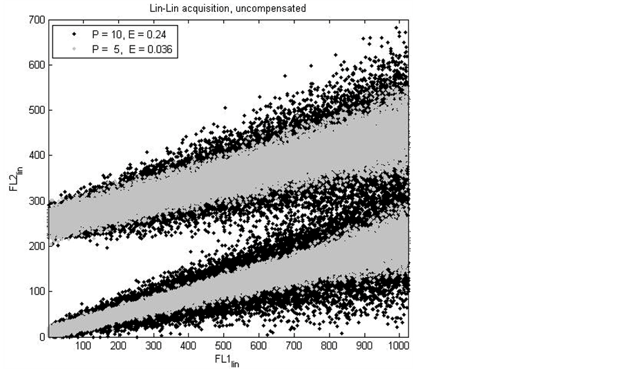
Figure 1. An overlay of two dot plots of two parameter, modelled flow cytometry experiments. One experiment with error term P = 10 (counting statistics) and error term E = 0.24 (measurement error and log scale binning error) (black dots) and one experiment with error term P = 5 and E = 0.036 (grey dots), see Equation (4), Equation (5) and Section 2.3. The FL1 parameter values are evenly distributed from 1 to 1024 in the linear domain (FL1lin, abscissa). The FL2 parameter values are separated in two Gaussian distributions in the linear domain (FL2lin, ordinate). This separation is caused by positive and negative FL2 parameter values. The slope of the distributions is caused by a correlation between the FL1lin and the FL2lin parameter, introduced by spectral cross-over (model compensation value “s” = 0.2). The plots show different values for the error terms P and E. Both error terms determine the magnitude of the broadening of the FL2 distribution, which is correlated with increasing FL1 intensity [5] . The magnitude of the broadening decreases with decreasing values for the error terms.
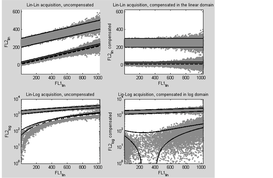
Figure 2. Four dot plots of modelled fluorescence intensity values of a primary detector (FL1) and a secondary (cross-over) detector (FL2). The model simulates a two parameter flow cytometry acquisition with 20% spectral cross-over from the primary parameter 1 (abscissa) into the secondary parameter 2 (ordinate). Each plot shows two distributions of grey events, one negative for parameter 2 (lower distribution) and one positive for parameter 2 (upper distribution). All values for the primary parameter are expressed in the linear domain. The upper two dot plots show the values of the secondary parameter in the linear domain. In the lower plots these linear values are logarithmic transformed and rescaled. The black dashed and the white dot dashed lines, represent the compensation trace lines and the four black lines represent predefined threshold lines. The top left plot shows the uncompensated modelled events. The top right plot shows the modelled events compensated in the linear domain. The lower left figure shows the uncompensated modelled events after logarithmic transformation and rescaling of parameter 2. The lower right figure shows the result of compensating the modelled events in the semilogarithmic domain.
shold line is between the upper bound and the black striped compensation trace line. All four threshold lines are parallel to the compensation trace line.
The second plot (top right) shows the modelled events and threshold lines, compensated in the linear domain. The upper horizontal shows the positive grey events and is still bounded by two of the threshold lines. Since these threshold lines are parallel to the striped compensation trace line, this indicates proper compensation. The lower horizontal shows the negative grey events with also two threshold lines. These threshold lines are also on a horizontal. Although the events and threshold lines are proper compensated (model compensation value, s = 0.2000, calculated compensation value, a = 0.2003), the intensity dependant broadening of the events remains. The mean percentage events that became less than zero after compensation, based on 10 experiments, is 9.29% with a standard deviation of 0.19.
The third plot (bottom left) is the same as the first plot except for the parameter values from the FL2 detector which were logarithmically transformed and rescaled. Compensation was then performed in the logarithmic domain, using the recalculated compensation value (model compensation value, s = 0.2000 and recalculated compensation value, a = 1.14).
The fourth plot (bottom right) represents classical compensation in the lin-log domain. The upper diagonal, containing the positive grey events, shows an intensity dependant broadening and an intensity dependant bias. The intensity dependant bias is seen in the slope of the two threshold lines that bound the upper diagonal. The events on the lower grey diagonal are scattered, and the two threshold lines are deformed. Both the deformation of the two threshold lines and scattering of the grey events is the most explicit between values 200 and 400 of the FL1 intensity, which corresponds to the S-phase area of a DNA histogram. The mean percentage events that became less than zero after compensation, based on 10 experiments, is 33.28% with a standard deviation of 0.13. The height of the compensated compensation trace line is near zero and can therefore not be seen in this logarithmic display where the ordinate starts at 1 (100).
3.2. Compensation Trace lines
The results in figure 2 show a discrepancy between the dot plot compensated in the linear domain and the one compensated in the semi-logarithmic domain. The reason for this discrepancy is the use two different compensation trace lines for compensation. The first compensation trace line is fitted through the negative distribution of the modelled events in the linear domain (figure 2, top left, dashed line). The second compensation line is fitted through the negative distributed events in the semi-logarithmic domain (figure 2, lower left, white dot dashed line). As explained before these negative events are ideal to fit the optimal compensation trace line. Although in both cases a first order equation is used for fitting Equation (6), the values and distribution of the FL2 parameter (ordinate) differ. Therefore the fitted compensation trace lines have different slopes. This is shown in figure 3, with the dashed and the dot dashed lines. The dashed line is fitted through the negative population of the events in the linear domain. The dot dashed line is fitted through the negative population of events in the semi-logarithmic domain. The slope, and therefore also the compensation value, increases from 0.2 in the linear domain to 1.14 in the semi-logarithmic domain. The latter compensation value exceeds 100%.
Instead of logarithmically transforming and rescaling the FL2 parameter values of the events used to fit a compensation trace line, the FL2 values of the compensation trace line can also be logarithmically transformed and rescaled. When these FL2 values from the compensation line, fitted in the linear domain, are logarithmic transformed and rescaled, the compensation line becomes curved. This is shown in figure 3, with the straight line. This straight line curves around the dot dashed line, which is traditionally used to compensate events in the semi-logarithmic domain [2] . Where the dot dashed line is above the straight line, overcompensation of the data in the semi-logarithmic domain occurs. Where the straight line is above the dot dashed line, under compensation in the semi-logarithmic domain occurs. This explains the distribution of the compensated events in figure 2, bottom right.
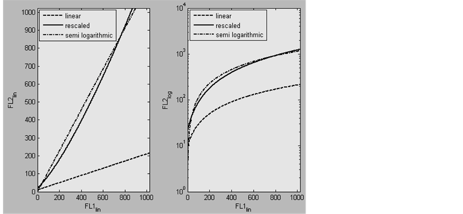
Figure 3. Two plots of compensation trace lines that can be used to compensate the modelled data in experiment 1 (see text). FL1lin and FL2lin are linear distributed parameter values and FL2log are logarithmically transformed and rescaled parameter values. The left plot shows 3 compensation trace lines in the linear domain, the right plot shows the same lines in the semilogarithmic domain. The dashed line is fitted through the negative events of the data which is modelled in the linear-domain. The dot dashed line is fitted through the negative events of the data of which the FL2 values were logarithmically transformed and rescaled. The continuous line is the result of logarithmically transforming and rescaling the FL2 values of the dashed compensation trace line.
3.3. Experiment 2
The purpose of the next experiment is to validate the results of experiment 1, with a real world example. This real world example consists of a set of two parameter acquisitions. One of these served as isotype negative control and the other as test sample. Both acquisitions were compensated twice; once in the lin-log domain, displayed in figure 4(1A) & figure 4(1B) and once in the lin-lin domain displayed in figure 4(2A), figure 4(2B), figure 4(3A) & figure 4(3B). The difference between the figure 4(2) & figure 4(3) is that the FL2-lin parameter is logarithmically transformed and rescaled to the logarithmic domain, after compensation.
In all dot plots in figure 4, two main distributions can be separated at FL1-PI intensities of 200 (2C peak) and 400 (4C peak). In the linear domain (figure 4(2A) & figure 4(2B), these distributions are flattened compared to the ones with logarithmically transformed and rescaled FL2-FITC parameter values. Despite the flattening, all the test samples show positive events in the 2C distribution compared to the isotype negative control. The 4C peak shows a difference between figure 4(1A) & figure 4(3A) with the latter being more dense. In the S-phase region of the dot plots (between the 2C and 4C peaks) the difference in density between the upper (figure 4(1A) & figure 4(1B) and lower (figure 4(3A) & figure 4(3B) plots is even more pronounced. The lower plots show a more dense and sharp edged S-phase region, compared to the upper plots.
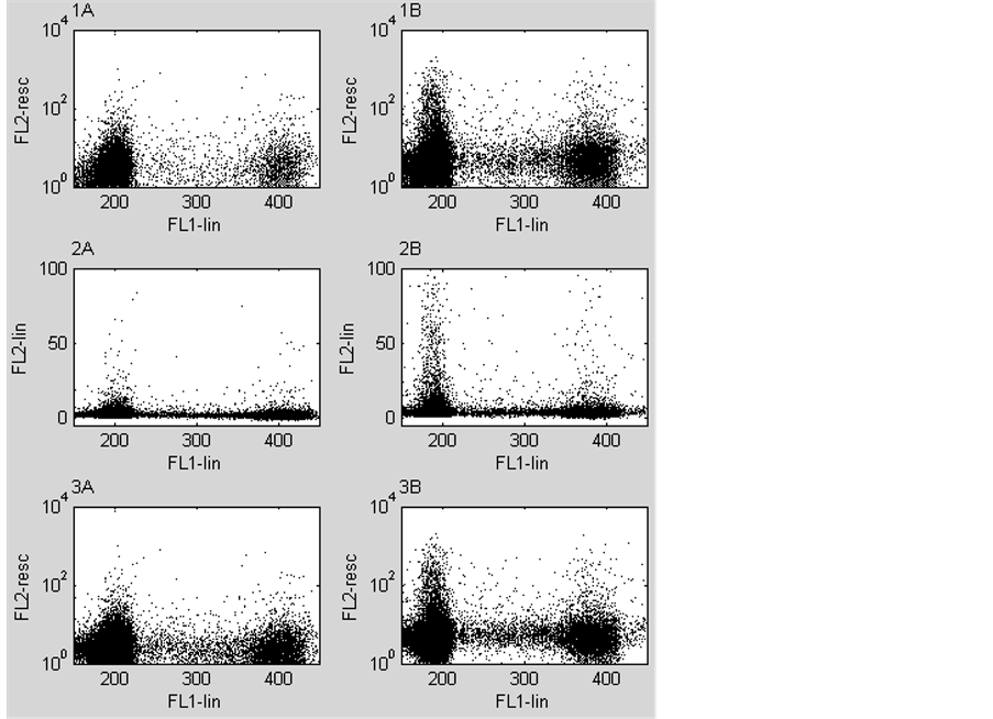
Figure 4. Six dot plots of two flow cytometry acquisitions, the left ones are from a negative control sample and the right ones are from a test sample. The negative control contains the fluorochromes PI (FL1-lin) and a mouse isotype negative control labelled with FITC. The test sample contains also PI and a MNF-116 labelled FITC. Dot plots 1A&B are the result of traditional compensation of a logarithmically transformed and rescaled parameter (FL2-resc) for overlap of a linear distributed parameter (FL1-lin). Dot plots 2A&B are the result of compensation of two linear distributed parameters of which the FL2-lin parameter is recalculated from the logarithmic to the linear domain. Dot plots 3A&B are the same as dot plots 2A&B with the exception that the FL2-lin parameter is logarithmically transformed and rescaled to it’s original domain after compensation. The samples contain single cells from a diploid lymph node metastasis. The cells in G0/G1-phase of the cell cycle are distributed around position 200 of the abscissa (2C peak). The cells in the combined G2 and M-phase of the cell cycle are distributed around position 400 (4C peak) and the cells in the S-phase are in between the two main distributions. For visibility the graphs show only the diploid part of the distributions.
The percentage events that became less than zero after compensation is for figure 4(1A), 58.5% and for Figure 4(1B), 8.2%. These percentages are respectively 1.7% and 0.1% for Figure 4(2A) & Figure 4(2B) and for figure 4(3A) & figure 4(3B).
A more dense S-phase region in the negative control makes it more suitable to set accurate thresholds for comparison with the test sample.
4. Discussion
The goal of this paper is to compare the results of spectral compensation of two linear distributed parameters, with the situation in which the parameter that has to be compensated is logarithmically transformed and rescaled. The main reason to do so was that we found compensation values in two and three colour acquisitions that were theoretically not possible, when one of the parameters was linear distributed. We adapted an existing flow cytometrie model to understand the extreme high compensation values. With this flow cytometry model two main differences were found between compensation in the lin-lin and the lin-log domain. 1) The compensation value in the linear domain equals the theoretically expected value (i.e. model compensation value). The compensation value in the lin-log domain exceeds 100%. A compensation value exceeding 100% is theoretically impossible because it means that a fluorochrome causes a higher secondary cross-over signal than it’s primary signal. This should indicate that the selection of the optical filters before the PMT’s is incorrect. However, it is shown that the compensation value only exceeds 100% after logarithmically transformation and rescaling of one parameter. The reason for this is that logarithmic transformation and rescaling leads to a factor 10 increase of parameter values compared to linear parameter values. The compensation value is defined as the slope of the optimal compensation trace line between two parameters. Increasing the values of one of the two parameters leads therefore to an increase of the slope of the compensation trace line. 2) Traditional compensation in the lin-log domain leads to deformation of the compensated events, compared to compensation in the lin-lin domain. While the optimal compensation trace line in the lin-lin domain is linear (y = a × x + b) we’ve shown that the optimal compensation trace line in the lin-log domain is curved. This curve is introduced by the non-linear logarithmic transformation of one parameter. Thus, when a traditional linear compensation trace line is used to compensate in the lin-log domain, it will lead to deformation of the distribution of compensated of events. This deformation makes that compensated events accumulate on the linear axes, especially in the S-phase region of a DNA acquisition. The second experiment, with the real world example, confirmed all the results that were obtained in the experiments with the model i.e. an increase in compensation value and an increase in the number of events that accumulate on the axes after logarithmic transformation and rescaling of one parameter.
Despite all the advantages of flow cytometry, spectral compensation is time consuming and very difficult to do manually, because there is only a subjective criterion for correct compensation. This criterion is a horizontal or vertical distribution of negative events after compensation [10] . When compensated events are deformed by the compensation process, this criterion for evaluation of a correct manual compensation does not hold anymore. This makes lin-log acquisitions impossible to compensate manually, using a linear compensation trace line. Hardware based compensation in our flow cytometer is done on linear distributed integers, before logarithmic amplification. Although hardware compensation is processed in the lin-lin domain, the disadvantage is that it can lead to over or under compensation because the correct median fluorochrome intensity can not be calculated, as is explained in [1] . Automated software based spectral compensation is fast, simple and in view of the difficulties mentioned above, tempting to accept in routine. However, automated compensation is executed in a black box, because all known suppliers of compensation software use their own algorithms. We have shown in our experiments that current available compensation algorithms do not work correctly in the lin-log domain. The resulting deformation of compensated events can not be seen in the compensation results, because the compensated events accumulate on the axis. With the formulae in this paper, automated compensation algorithms can be adapted to correctly compensate events in the lin-log domain using a curved compensation trace line. Our experiments also demonstrate that there is no need for logarithmic transformation and rescaling of linear data. The compensation results of using a linear compensation trace line in the lin-lin domain are exactly the same as using a curved compensation trace line in the lin-log domain. While the latter has the huge disadvantage that on one axis no negative events can be displayed. Just like we proved that a linear compensation trace line in the lin-log domain yields deformation of compensated events, it is also possible to prove that a linear compensation trace line in the log-log domain yields deformation of compensated events in the first and fourth log decade. Once the idea is accepted that a linear compensation trace line can be calculated and applied in the linear domain, automated compensation can be done reliably, fast and reproducible on linear datasets after acquisition. The proposed compensation approach can also be applied to uncompensated historical data and re-compensation might result in new insight on the use of data from the S-phase region in DNA flow cytometry.
References
- Bagwell, C.B. and Adams, E.G. (1993) Fluorescence Spectral Overlap Compensation for Any Number of Flow Cytometry Parameters. Annals of the New York Academy of Sciences, 677, 167-184. http://dx.doi.org/10.1111/j.1749-6632.1993.tb38775.x
- Corver, W.E., Fleuren, G.J. and Cornelisse, C.J. (2002) Software Compensation Improves the Analysis of Heterogeneous Tumor Samples Stained for Multiparameter DNA Flow Cytometry. Journal of Immunological Methods, 260, 97-107. http://dx.doi.org/10.1016/S0022-1759(01)00550-6
- Maecker, H.T. and Trotter, J. (2006) Flow Cytometry Controls, Instrument Setup, and the Determination of Positivity. Cytometry A, 69, 1037-42. http://dx.doi.org/10.1002/cyto.a.20333
- Roederer, M. (2002) Compensation in Flow Cytometry. Current Protocols in Cytometry, 22, 1.14.1-1.14.20.
- Roederer, M. (2001) Spectral Compensation for Flow Cytometry: Visualization Artifacts, Limitations, and Caveats. Cytometry, 45, 194-205. http://dx.doi.org/10.1002/1097-0320(20011101)45:3<194::AID-CYTO1163>3.0.CO;2-C
- Stewart, C.C. and Stewart, S.J. (1999) Four Color Compensation. Cytometry, 38, 161-175. http://dx.doi.org/10.1002/(SICI)1097-0320(19990815)38:4<161::AID-CYTO3>3.0.CO;2-A
- Stewart, C.C. and Stewart, S.J. (2003) A Software Method for Color Compensation. Current Protocols in Cytometry, Chapter 10, Unit 10 15.
- Tung, J.W., Parks, D.R., Moore, W.A., Herzenberg, L.A. and Herzenberg, L.A. (2004) New Approaches to Fluorescence Compensation and Visualization of Facs Data. Clinical Immunology, 110, 277-283. http://dx.doi.org/10.1016/j.clim.2003.11.016
- Verity Software House, Inc. (2002) A Discussion of Linear-to-Log Data Conversion in Flow Cytometry. Topsham, 1-6. http://ftp.vsh.com/publication/LinLog.pdf
- van Rodijnen, N.M., et al. (2011) Data-Driven Compensation for Flow Cytometry of Solid Tissues. Advances in Bio-informatics, 2011, Article ID: 184731. http://www.hindawi.com/journals/abi/2011/184731/abs/
- Radcliff, G. and Jaroszeski, M.J. (1998) Basics of Flow Cytometry. Methods in Molecular Biology, 91, 1-24.
- Roederer, M., De Rosa, S., Gerstein, R., Anderson, M., Bigos, M., Stovel, R., Nozaki, T., Parks, D., Herzenberg, L. and Herzenberg, L. (1997) 8 Color, 10-Parameter Flow Cytometry to Elucidate Complex Leukocyte Heterogeneity. Cytometry, 29, 328-339. http://dx.doi.org/10.1002/(SICI)1097-0320(19971201)29:4<328::AID-CYTO10>3.0.CO;2-W
- Leers, M.P., Schoffelen, R.H.M.G., Hoop, J.G.M., Theunissen, P.H.M.H., Oosterhuis, J.W.A., vd Bijl, H., Rahmy, A., Tan, W. and Nap, M. (2002) Multiparameter Flow Cytometry as a Tool for the Detection of Micrometastatic Tumour Cells in the Sentinel Lymph Node Procedure of Patients with Breast Cancer. Journal of Clinical Pathology, 55, 359-366. http://dx.doi.org/10.1136/jcp.55.5.359
- Leers, M.P., Schutte, B., Theunissen, P.H.M.H., Ramaekers, F.C.S and Nap, M. (1999) Heat Pretreatment Increases Resolution in DNA Flow Cytometry of Paraffin-Embedded Tumor Tissue. Cytometry, 35, 260-266. http://dx.doi.org/10.1002/(SICI)1097-0320(19990301)35:3<260::AID-CYTO9>3.0.CO;2-O
- Leers, M.P., Theunissen, P.H.M.H., Schutte, B. and Ramaekers, F.C.S. (1995) Bivariate Cytokeratin/DNA Flow Cytometric Analysis of Paraffin-Embedded Samples from Colorectal Carcinomas. Cytometry, 21, 101-107. http://dx.doi.org/10.1002/cyto.990210118