Atmospheric and Climate Sciences
Vol.3 No.4(2013), Article ID:37965,14 pages DOI:10.4236/acs.2013.34059
Source Apportionment of PM2.5 in the Metropolitan Area of Costa Rica Using Receptor Models
1Laboratorio de Análisis Ambiental, Escuela Ciencias Ambientales, Universidad Nacional, Heredia, Costa Rica
2Escuela de Química, Universidad de Costa Rica, Ciudad Universitaria Rodrigo Facio, Costa Rica
3DGCENICA, Instituto Nacional de Ecología, México DF, México
Email: *jorge.herrera.murillo@una.cr
Copyright © 2013 Jorge Herrera Murillo et al. This is an open access article distributed under the Creative Commons Attribution License, which permits unrestricted use, distribution, and reproduction in any medium, provided the original work is properly cited.
Received June 4, 2013; revised July 5, 2013; accepted July 13, 2013
Keywords: PM2.5; Chemical Composition; Costa Rica; Source Apportionment; Receptor Models
ABSTRACT
In this work, receptor models were used to identify the PM2.5 sources and its contribution to the air quality in residential, comercial and industrial sampling sites in the Metropolitan Area of Costa Rica. Principal component analysis with absolute principal component scores (PCA-APCS), UNIMX and positive matrix factorization (PMF) was applied to analyze the data collected during 1 year of sampling campaign (2010-2011). The PM2.5 samples were characterized through its composition looking for trace elements, inorganic ions and organic and elemental carbon. These three models identified some common sources of PM2.5: marine aerosol, crustal material, traffic, secondary aerosols (secondary sulfate and secondary nitrate resolved by PMF), a mixed source of heavy fuels combustion and biomass burning, and industrial emissions. The three models predicted that the major sources of PM2.5 in the Metropolitan Area of Costa Rica were related to anthropogenic sources (73%, 65% and 69%, respectively, for PCA-APCS, Unmix and PMF) although natural sources also contributed to PM2.5 (21%, 24% and 26%). On average, PCA and PMF methods resolved 94% and 95% of the PM2.5 mass concentrations, respectively. The results were comparable to the estimate using UNMIX.
1. Introduction
The atmospheric particulate matter (PM) consists of particles which have their origin by several sources and processes, such as direct emissions from mobile sources, space heating, metal processing, refuse incineration, erosion and resuspension, gas-to-particle conversion and long range transport. PM is composed of inorganic salts, organic material, crustal elements and trace metals and possess a range of morphological, physical, chemical and thermodynamic properties. Airborne particles can change in the atmosphere in size and/or composition through condensation of vapor species or by evaporation, by coagulating with other particles, by chemical reaction, or by activation in the presence of supersaturated water vapor to become cloud and fog droplets [1].
The sources, characteristics and potential health effects of the larger or coarse particles (>2.5 µm in diameter) and smaller or fine particles (<2.5 µm in diameter) are very different. Many studies indicate that the fine aerosol fractions have the greatest impact on health because they can go all the way into the respiratory tract, inducing chronic respiratory illness, asthma, cancer and premature dead [2,3]. PM concentrations have been routinely monitored. However, this level of monitoring is insufficient and a measurement of the elemental and chemical composition of PM is recommended.
One of the main difficulties in air pollution management is to determine the quantitative relationship between ambient air quality and pollutant sources. Source apportionment is the process of identification of aerosols emission sources and quantification of the contribution of these sources to the aerosol mass and composition. Identification of pollutant sources is the first step in the process of devising effective strategies to control pollutants. After sources are identified, characterization of the source’s emission rate and emission inventory can be followed by the development of a control strategy including the possibility of revised or new regulations.
Under the supposition that chemical components found in a given ambient sample, have a strong correspondence to the chemical composition of the source emissions, during last years, receptors models have been one of the most important tools in source apportionment studies [4-7]. All receptor models use ambient air measurements of the different chemical species to infer the source types, locations and contributions that affect ambient pollutant concentrations. Receptor models allow correlation of the concentrations of measured chemical species in a site known as a receptor with the emission sources. Receptor models have been used to quantify source contributions to PM10 and PM2.5, identify un-inventoried sources, improve emission inventories and track the long term effectiveness of pollution control strategies [8].
While source models need spatial and temporal resolution and accurate emissions rates, receptor models need only a seasonal or annual average wide area inventory to identify potential source categories. Receptor models are based on the chemical mass balance (CMB) principle where the main assumption is that the composition of PM remains constant and the chemical species do not react with each other. CMB equations may be solved by effective variance (EV), Positive Matrix Factorization (PMF), or Unmix methods [9]. The EV-CMB solution uses both source profiles and ambient concentrations as inputs and calculates source contribution estimates (SCEs) and their uncertainties for individual samples. The PMF-CMB and Unmix-CMB solutions derive source factors and contribution estimates simultaneously from a time series and/or spatial distribution of ambient measurements, and then associate these factors with source types by comparison with measured source profiles. Validation tests are specified for the EV-CMB solution that have not been adapted or applied yet to the PMF or Unmix solutions. Comparison of SCEs from these solutions provides an independent validation test, consistent with the “weight of evidence” approach to SCEs. In addition, a CMB solution should be consistent with the conceptual model, or reasonable modifications to the conceptual model are revealed [10].
The objectives of the present paper are to 1) analyze the concentration and chemical composition distribution of atmospheric PM2.5 at five sites in the Metropolitan Area of Costa Rica and 2) compare the results of three different receptor models used for the characterization of potential PM2.5 sources.
2. Methodology
2.1. Study Area Description
The study was carried out in the Metropolitan Area of Costa Rica located in a central plateau of around 3000 km2 surface within a mountain system that cross the country from NW to SE, with peaks with a maximum height of around 4000 meters (Figure 1). The metropolitan area is the highest-ranking center in the urban system in Costa Rica, accounting for 75% of the vehicle fleet (approximately 734,200 units), 65% of the domestic industry and 60% of the country's population (2,580,000), according to data from the last population census conducted in 2010. Lack of urban planning have led to an accelerated deterioration of air quality, as a result of growth experienced by the cities of the Metropolitan Area of Costa Rica during the past 20 years.
2.2. Sampling
For the PM2.5 sampling, five monitoring sites were selected (Table 1). The sites were representative of com-

Figure 1. Location of the sampling sites in the Metropolitan Area of Costa Rica.
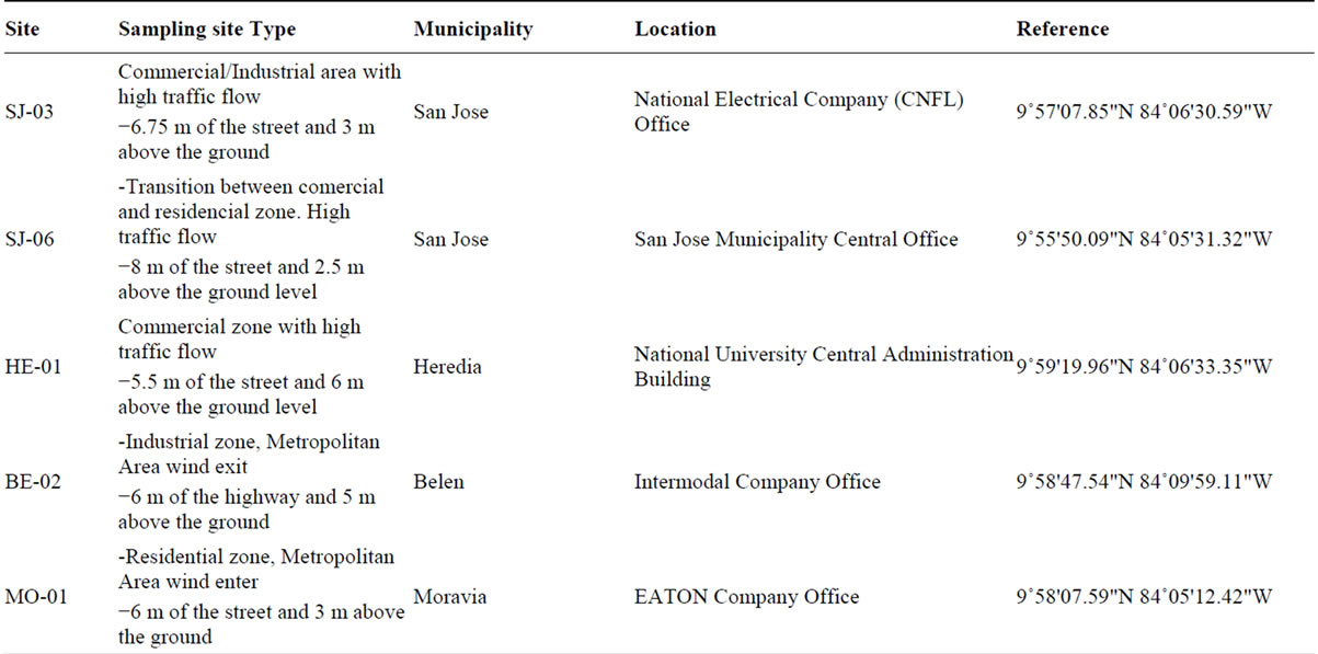
Table 1. Description of sampling sites used in the PM2.5 analysis.
mercial, industrial and residential areas, all located in the Costa Rica metropolitan area. Sampling campaign was conducted between May 2010 and July 2011. Samples were collected once each three days for a total of 110 by sampling site. To collect the samples, two low volume air samplers, Air Metrics were used with a flow rate of 5 l min−1in each sampling site. The separation of the PM2.5 fraction takes place at the entrance of the sample by a head with two impactors, one (located on the top) that separates the total PM10 and a second impactor that separates the fraction of PM2.5 particles of the PM10. PM2.5 samples were collected on 47-mm Teflon membrane filters (nominal pore size 2 μm) (Pall Corporation, Ann Arbor, MI, USA) and 47-mm quartz filters (Pallflex TYPE:Tissuquartz 2500QAT-UP002C Clifton, NJ, USA). Samples were collected during 24 h on a pre-fired (at least 5 h at 900˚C) quartz fibre filters (Pallflex TYPE: Tissuquartz 2500QAT-UP). Before and after collection, the samples were stored in the freezer and they were also kept frozen during transport. After particle collection, the Teflon membrane filters were reconditioned for another 24 h in an air conditioned room and subsequently analysed for total mass. After sampling, the exposed quartz filters were stored in a freezer at −5˚C to limit losses of volatile components. Special care was taken during the handling of the filters to avoid any possible contamination.
2.3. Chemical Analysis
Samples collected in Teflon membrane filters were used for gravimetric analysis in order to determinate the PM2.5 concentrations. The weighing of the low volume filters was performed using a semimicroanalytic balance (Mettler). The readability of the balance is 10 mg with a precision of ±40 mg corresponding to mass concentration uncertainty of ±0.86 mg/m3 for PM2.5 samples. They were weighed at least three times to obtain constant values.
Quartz filters were cut in three equal parts to analyse chemical composition. A small portion of quartz filters were analyzed for Organic Carbon (OC) and Elemental Carbon (EC) using DRI Model 2001 Thermal/Optical Carbon Analyzer (Atmoslytic Inc., Calabasas, CA, USA). A 0.68 cm2 punch from each filter was analyzed for eight carbon fractions following the IMPROVE TOR protocol. This produced four OC fractions (OC1, OC2, OC3, and OC4 at 120˚C, 250˚C, 450˚C, and 550˚C, respectively, in a helium atmosphere), a pyrolyzed carbon fraction (OP, determined when reflected laser light attained its original intensity after oxygen was added to the combustion atmosphere), and three EC fractions (EC1, EC2, and EC3 at 550˚C, 700˚C, and 800˚C, respectively, in a 2% oxygen and 98% helium atmosphere). IMPROVE OC is operationally defined as OC1 + OC2 + OC3 + OC4 + OP and EC is defined as EC1 + EC2 + EC3 − OP. For the OC and EC determination, the analyzer was calibrated using different aliquots (0, 3, 5, 7, 10, 12, 15, 20 and 25 ml) of a standard sucrose solution (4260 mg/l) over a filter blank (pre-heated Quartz filter punch). The detection limits (LODs) for OC and EC were 746 ngm−3 and 180 ngm−3, respectively. Analytical uncertainties for OC and EC were estimated to be 16% and 9%, respectively. NIST 8785 reference material was used in order to evaluate the analytical method accuracy for the determination of organic and elemental carbon in PM2.5. This reference material consists in a thin fraction of SRM 1649 (Urban Dust) deposited on a quartz fiber filter. Seven replicates of NIST 8785 were analized and the results are showed in Table 2. There is not a significative difference between obtained values and reference values, a confidence level of 95%, according to a t test for medians comparation.
Another filter portion was extracted in 50 ml desionized water during 35 minutes in an ultrasonic bath. The analysis of ionic species was performed by dual microbore suppresed Ion Chromatography using a DIONEX ICS-3000 equipment with a quaternary pump. A fresh calibration curve were prepared for every 20 samples, together with a dissolution of quality control of 5 mg·l−1 prepared from a certified DIONEX synthetic sample. Detection limits for each ion are shown in Table 3.
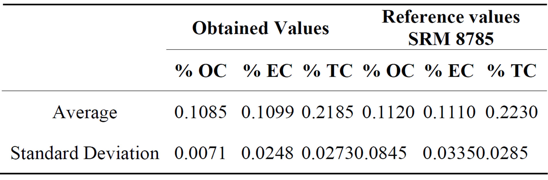
Table 2. Results of SRM 8785 reference material analysis for Organic carbon and elemental carbon percent aje.
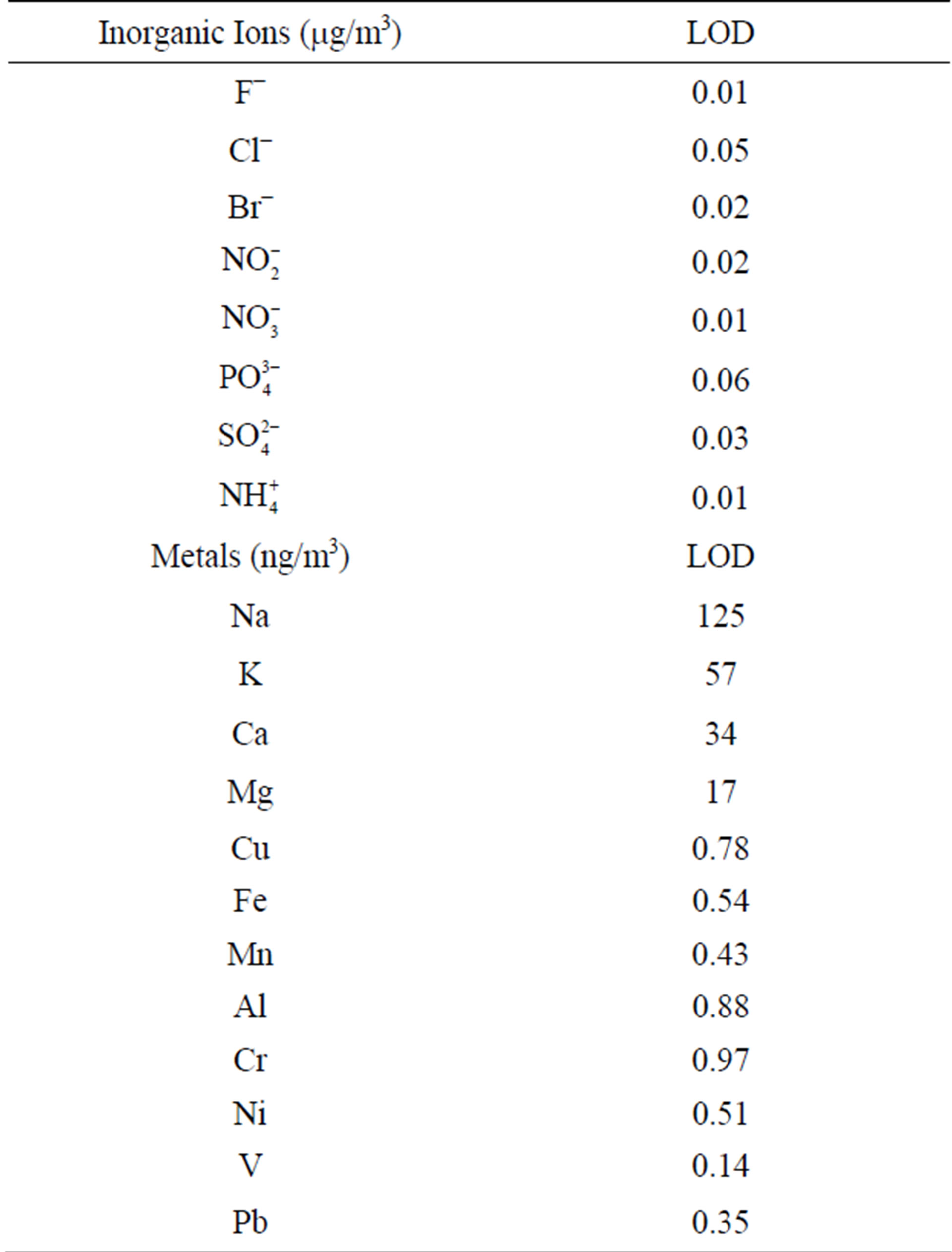
Table 3. Limit of detection (LOD) of different chemical species analyzed in PM2.5.
The last filter portion was extracted adding 5 ml of ultra-pure concentrated nitric acid and 25 ml of desionized water and heated on a hot plate until almost dryness. The remaining solution was poured into a 25 ml volumetric flask. A second extraction was done with 1 ml of concentrated HClO4. Metals analysis was made using graphite furnace atomic absorption spectroscopy (PERKIN ELMER AANALYST 700). Detection limits in ngm−3 were obtained according IUPAC method [11]. The results are shown in Table 3. Blank filters were analyzed for metals and inorganic ions, obtaining concentrations about 5% lower than those found in samples. The accuracy of the metal chemical analysis was periodically checked using a certified standard (SRM 1648) for blank filter enrichment. An overall bias between −8% and 13% was obtained for metal concentrations measured in enrichment samples.
Finally, contents of Si and  were indirectly determined from the contents of Al, Ca and Mg, on the basis of previous experimental equations (Al × 1.89 = Al2O3, 3Al2O3 = SiO2; 1.5Ca + 2.5Mg =
 ) [12].
2.4. Receptor Models
The 2007 Costa Rica Metropolitan Area criteria pollutant emission inventory [13] attributed 60.8% of primary PM2.5 emission to non-point (area) sources, followed by mobile sources (26.7%) and point (12.5%) emitters. Non-point sources include fugitive dust emissions from paved roads, unpaved roads, and agricultural tilling, as well as residential waste burning emissions, prescribed burning, and wildfires. Although the authors identified the source types that might contribute to ambient PM2.5, they do not have information about the specific sources profiles. PCA-APCS, UNMIX and PMF were applied to the collected data in order to estimate source profiles and contributions.
Principal Component Analysis (PCA) model belongs to the category of factor analysis (FA) techniques, i.e. it is a multivariate method used to study the correlations among the measured chemical concentrations at the receptor. With this method, the principal components explain the observed variance of the data for the analyzed chemical species, and then it’s interpreted to identify possible sources. The main objective of PCA is to reduce a large number of variables to a smaller set of factors that retain most of the information (variability) from the original dataset [14]. To ensure that both elements with low or high concentrations are treated equally, PCA requires the original variables to be normalised and dimensionless.
 (1)
(1)
where: i = 1, ···, m elements and j = 1, ···, n samples, zij is the reduced mass concentration of the ith element in the jth sample, xij is the ith elemental mass concentration measured in the jth sample, xi is the mean mass concentration of the ith element, σi is the standard deviation associated to the xi.
PCA assumes that the variables (here concentrations) are linearly-related to a number p of factors (assumed here to be the sources) so that the reduced concentration of each element is made up of the linear sum of elemental contributions from each pollution source at the recaptor site:
 (2)
(2)
where, aik is the factor loading of the ith element to the kth component (source) and ckj is the factor score of the kth component (source) to the jth sample. This equation is solved by eigenvector decomposition. Varimax rotation is often used to redistribute the variance and provide a more interpretable structure to the factors.
APCS (Absolute Principal Component scores) is then used, based on the PCA factor scores, to derive quantitative estimates of source contributions and source profiles [14]. Because the PCA results are based on normalized data, the true zero for each factor score should be calculated as:
 (3)
(3)
The rescaled scores are known as APCS. Finally, regression can be used to derive the source contributions, expressed as
 (4)
(4)
where Mi is the measured mass concentrations in sample i. APCSki is the rotated absolute component score for source k in sample i. ζkAPCSki is the mass contribution in sample i made by source k. ζ0 is the mass contribution made by sources unaccounted for in the PCA.
The UNMIX model is a refined multivariate receptor model that uses a new transformation method based on the self-modeling curve resolution technique to derive meaningful factors. UNMIX incorporates user-specified non-negativity constraints and edge-finding algorithms to derive a physically reasonable apportionment of source contributions [15,16].
The edges are constant ratios among chemical components that are detected in multi-dimensional space. The ones detected by this model are translated into source profile abundances. This model doesn’t require a previous knowledge about emission sources, although it is necessary a big number of measurements to estimate the different factors, as well as the magnitude of their contributions [16,17].
The first step adopted is applying “NUMFACT” to determine the number of influencing sources. This is analogous to factor analysis methods that establish the number of factors (or sources), but with different criteria being invoked. Singular value decomposition (SVD) is then performed on the normalized measured chemical concentration data to reduce the dimensions related to the retained number of factors (or sources). Once the edges of the data set are established, they are used to determine the source profiles. Contributions of these source categories can be calculated using the singular value decomposition model.
The PMF model is a multivariate receptor model that has been described in detail by [18] and implemented in the PMF2 program, which doesn’t require source profile knowledge unlike traditional source receptor models (CMB). This program is now being widely used to analyze airborne particulate matter sources [19-21].
PMF is a receptor model based on the principle that a relationship between sources and receptor exists when mass conservation can be assumed [22]. In this case, and when chemical speciation of ambient PM is available, a mass balance equation of the following form can be written:
 (5)
(5)
where xij is j-th species in the i-th sample. The mass fraction of species h in source i is ih a (e.g. source composition) and fhj is the total mass of material from source h in the j sample (e.g. source contribution). Obviously, equation above represents the general mixture problem and includes errors eij which may be the result of analytical uncertainty and variations in the source composition. The corresponding matrix equation is
 (6)
(6)
where X is a n × m matrix with n measurements and m number of elements. E is an n × m matrix of residuals. G is n × p source contribution matrix with p sources, and F is a p × m source profile matrix.
The signal-to-noise ratio (S/N) was used to select the species for further analysis. Species with S/N ratio below 0.2 were classified as bad values and were thus excluded from further analysis. The application of PMF depends on the estimated uncertainties for each of the data values. The uncertainty estimation provides a useful tool to decrease the weight of missing data and values below the detection limit data, in the solution. The procedure was used to assign measured data and the associated uncertainties as the input data to the PMF. The concentration values were used for the measured data, and the sum of the analytical uncertainty and 1/3 of the detection limit value was used as the overall uncertainty assigned to each measured value. Values below the detection limit were replaced by half of the detection limit values and their overall uncertainties were set at 5/6 of the detection limit values. Missing values were replaced by the geometric mean of the measured values and their accompanying uncertainties were set at four times of this geometric mean value. In addition, the estimated uncertainties of species that have scaled residuals larger than 72 need to be increased to reduce their weight in the solution [23].
3. Results and Discussion
3.1. PM2.5 Levels and Chemical Composition
The average PM2.5 concentrations at the 5 sites ranged between 18 and 37 mg/m3 (Table 4). The higher concentrations were found in high traffic commercial (HE-01) and industrial (BE-02) sites, 37 mg/m3 and 36 mg/m3, respectively. It was found that the PM2.5 concentrations in all the sampling sites were higher than 15 μg/m3, the US National Ambient Air Quality Standard. Daily concentrations exhibited 34% and 26% exceedances of the 24-h limit of the USA PM2.5 National Ambient Air Quality Standard (35 μg/m3) at the high traffic comercial (HE- 01) and the industrial site (BE-02), respectively. This indicates the need for local authorities to establish appropriate measures for PM emissions reduction. The comparation was done with USA standards due to Costa Rica doesn’t have an air quality standard for PM2.5, both daily and annual.
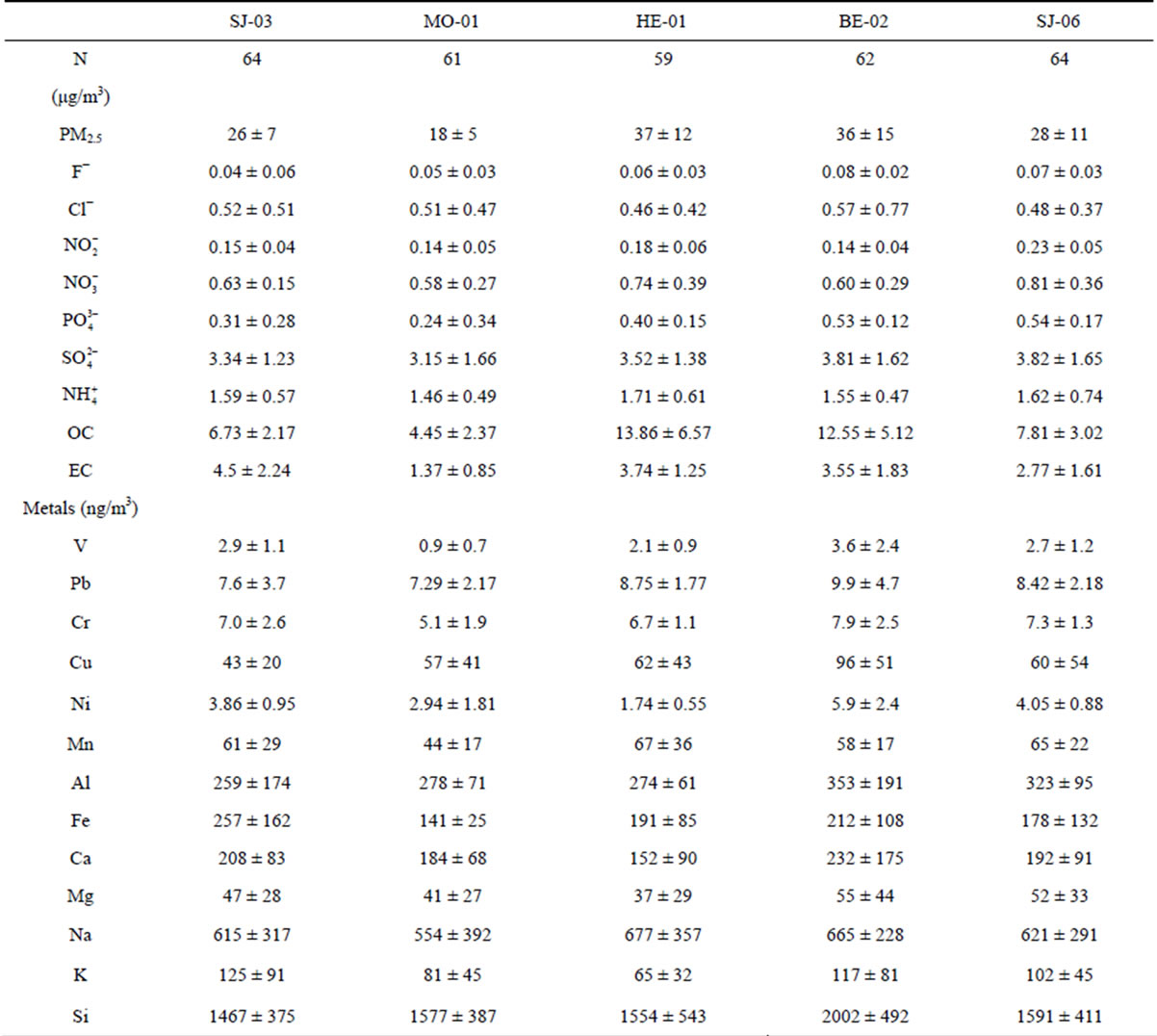
Table 4. Annual average PM2.5 levels and its chemical composition at the Metropolitan Area of Costa Rica (±standard deviation).
The largest mass contributions for all the sampling sites come from organic carbon (OC). OC is often emitted from burning sources, e.g., heavy fuels combustion and biomass burning, and from secondary organic aerosols (SOA). It is well know that many volatile organic compounds (VOCs) can suffer several photochemical reactions that can lead to the formation of SOA. The next important component (in absolute value) is sulphate, followed by elemental carbon (Figure 2).
Further clustering of components reveals that the ones related to total carbon matter (TCM) (OM + EC) are the most dominant. OM was obtained by multiplying the measured concentration of organic carbon (OC) by a factor of 1.6, which is based on an average of the recommended ratios (Turpin and Lim, 2001). This factor is commonly used to estimate the unmeasured hydrogen and oxygen in organic compounds. The TCM concentrations are higher at high traffic commercial and industrial sites (69.9% - 65.0%) whereas lower percentages are found at the residential stations (44.5%).
Organic carbon (OC), a mixture of hydrocarbons and oxygenates, is formed by a variety of processes, including combustion and secondary organic carbon (SOC) formation. The concentration of secondary organic carbon (SOC) can be estimated from:
 (7)
(7)
where OCsec is the secondary OC, and OCtot the measured total OC. The primary organic carbon (POC) could be calculated from the term “EC(OC/EC) primary”. However, the primary ratio of OC/EC is usually not available because it is affected by many factors such as the type of emission source as well as its variation in temporal and spatial scales, ambient temperature, and carbon determination method, etc. In many case, (OC/EC) primary was represented by the observed minimum ratio ((OC/EC) min), and assumptions regarding the use of this procedure as were discussed in detail by [24].
The annual average concentrations of estimated SOC in the Metropolitan Area of Costa Rica PM2.5 samples resulted in values between 2.31 to 7.01 mg/m3 (Table 5), accounting for 40% - 55% OC in PM2.5. Compared with rainy season results, there is an overall trend toward lower SOC levels but with a higher percentage of SOC in the TOC at each site during the dry season [25]. Higher

Table 5. Levels of SOC and POC obtained for PM2.5 samples in the Metropolitan Area of Costa Rica.
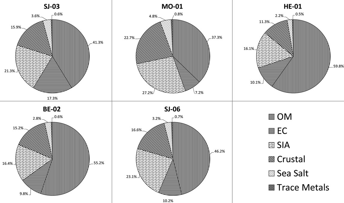
Figure 2. Chemical mass closure of PM2.5 at five sampling sites in the Metropolitan Area of Costa Rica.
temperatures and more intense solar radiation during the summer months provide favorable conditions for photochemical activity and SOC production.
The second dominant contribution to PM2.5 comes from secondary inorganic aerosol (SIA) (sum of ,
,  ,
, ): it ranges between 16.1% and 27.2% with a maximum at the residential area (MO-01). The contribution of the remaining components like sea salt (2.2% - 4.8%), crustal material (22.7% - 11.3%) and metals (0.5% - 0.8%) is relatively small in PM2.5 and rather independent of measurement site.
Crustal material contribution was calculated as the sum of typical crustal materials, including Al, K, Fe, Ca, Mg, Ti and Si. Each of these species was multiplied by the appropriate factor to account for its common oxides based on the following equation [11,26]:
CM = 1.89Al + 1.21K + 1.43Ca + 1.66Mg + 2.14Si.
The crustal contribution to PM2.5 mass increased from 11% - 13% in industrial and commercial areas to 23% in residential areas, this can be due to the existence of nonurban lands nearby. Because these regions are subjected to wind resuspension (or entrainment) processes. The resuspension of dust (crustal materials of diameter < 20 μm) by wind provides a potential source of particles to the atmosphere [11]
The Sea Salt contribution was computed as the sum of measured chloride ion concentration plus the sea salt fraction of concentrations of Na+, Mg2+, K+, Ca2+, . Additionally, metals contribution was estimated using the following equation: TE = 1.47[V] + 1.29[Mn] + 1.27[Ni] +1.25[Cu] +1.08[Pb] + 1.31[Cr]. The contribution of marine aerosol varies between 2% to 5% for sampling sites presenting a fairly regular basis. This evidences that the contribution of this component is due more to regional scale phenomena.
3.2. Source Identification with PCA
Principal component analysis was performed on the PM2.5 data sets of three sampling sites categories: residential (MO-01), commercial (HE-01, SJ-03, SJ-06) and industrial (BE-02), with the results shown in Table 6. A total of 18 variables were considered in the PCA with Varimax rotation, F− and  were excluded from the analysis because there isn’t a significative change of their levels in different samples so they won’t be sensitive to PCA. The lowest eigenvalue for extracted factors was restricted to more than 1.0. The analysis extracted four diferent factors for residential and five for commercial and industrial sampling sites (Table 6).
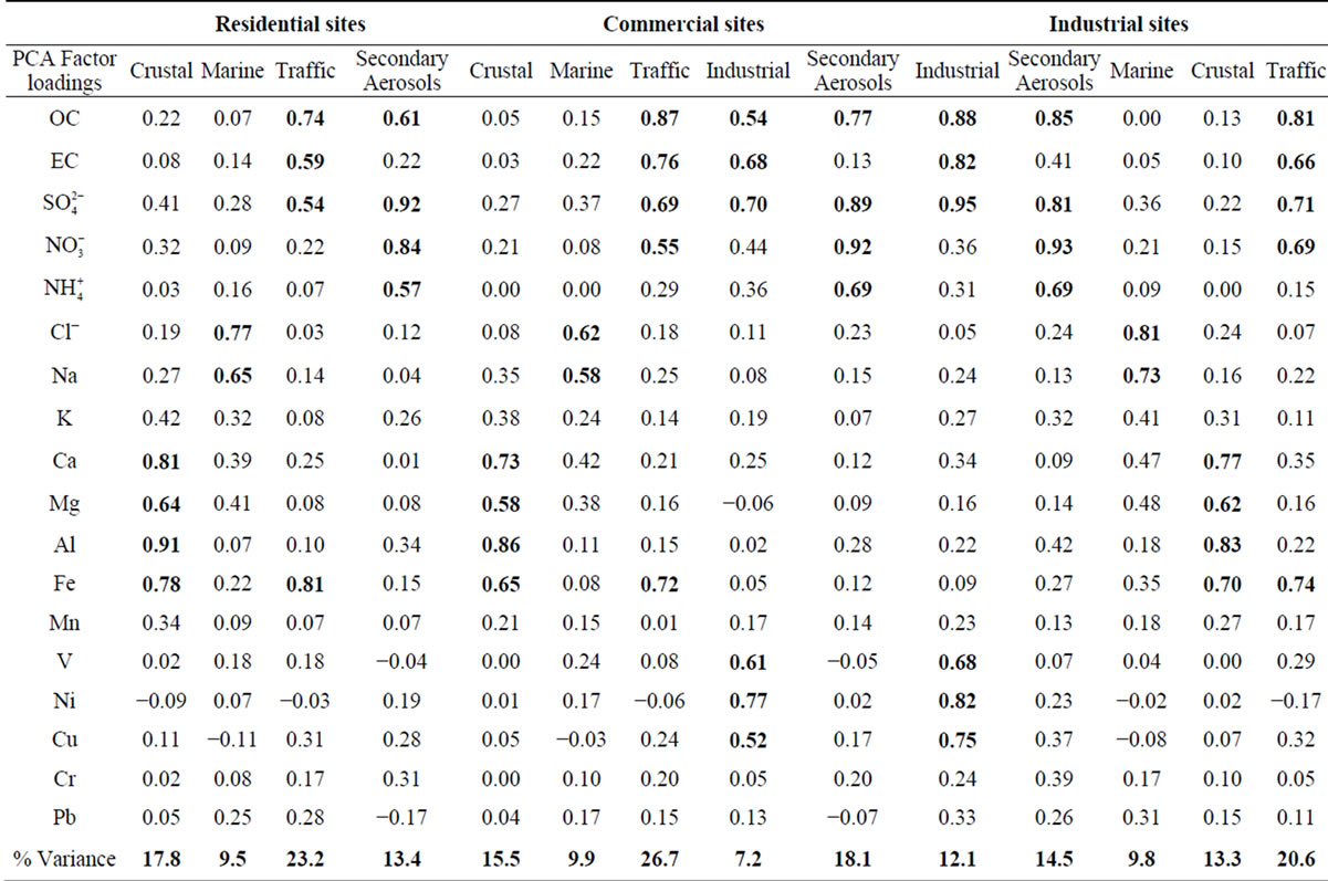
Table 6. PCA factor loadings for PM2.5 in residential, commercial and industrial sites.
3.2.1. Factor 1: Crustal
The crustal source is common to all the sampling sites, with Al, Fe, Ca and Mg as main tracers although other crustal elements such as K or Mn are also present. This factor represents the contribution of mineral particulate matter from natural (soil resuspension) and anthropogenic (construction activities, soil resuspension generated by traffic road, etc.) sources. The explained variance for this factor corresponds to 17.8% and 13.3% for residential and industrial sites, respectively.
3.2.2. Factor 2: Marine
This PM2.5 factor is present in all the sites. It takes into account the presence of Na and Cl and Mg in the particles. The latter is also a typical marine component (magnesium-sulfate) [27]. The percentage of variance explained by this factor is very similar in residential, commercial and industrial sites due to the contibution of regional wind patterns. Costa Rica is a narrow country that receives the influence of the Pacific Ocean and the Caribbean Sea. The Metropolitan Area is located in valley constantly ventilated by the winds coming from both sides, some of them dominate according to the season. This ensures a continuously renewal of the air and an input of marine aerosols.
3.2.3. Factor 3: Traffic
This factor was identified in all the sampling sites. It is constituted by components which are typically associated with the vehicle exhaust ( ,
, , OC, EC), road dust (Ca and Fe) and brake lining particles (Cu) [28]. A high percentage of the variance was better explained by this factor in commercial (26.7%) and residential (23.2%) than on industrial (20.6%) sites.
3.2.4. Factor 4: Secondary Aerosols
This is characterized by high sulfate, nitrate, and ammonium that could be identified as a mixture of secondary sulfate and secondary nitrate. These secondary products are often originated from the oxidation of SO2 and NOx and the neutralization of NH3 [29]. Also, the presence of OC explains the important contribution of SOA to the PM2.5 found at the sites. This is mainly produced by radical-initiated tropospheric reactions of hydrocarbons precursors, generating non-volatile and semivolatile organic products which lead both to particulate matter and nucleation reactions to form new particles.
Many studies have related the OC/EC ratio to secondary organic particle formation. A primary OC/EC ratio of 2.2 or 2.0 has been usually regarded as an indication of the presence of SOC [30]. In other words, the additional OC that causes the OC/EC ratio to exceed 2.2 or 2.0 can be considered to be secondary in origin. According to this hypothesis, SOC might play an important role in carbonaceous pollution in the MACR. The average OC/EC ratios at the sampling sites ranged from 1.40 - 3.96 for PM2.5. These values tend to be higher in the rainy season as compared to the dry season.
Another part of that OC comes from emissions of combustion activities which produce primary organic carbon (POC) as fine particles, typically PM2.5. The EC and OC PM2.5 inventory for the area includes a contribution of 8140 tons/year from OC and 2518 tons/year from EC. On an annual basis, the major sources of primary OC emissions are industrial combustion (92.3%), diesel vehicles (3.51%) and gasoline vehicles (2.65%). On an annual basis, the major EC sources are industrial combustion (74.7%), diesel vehicles (15.7%), residential combustion (5.4%) and gasoline vehicles (1.22%) [25].
The influence of this factor in the variance of the PM2.5 composition data was higher in commercial and Industrial sites due to the contribution of different combustion and area sources emissions, including SOA.
3.2.5. Factor 5: Industrial
This source could be a mixture of heavy oil combustion and biomass burning because PCA exhibited high levels for OC, EC, Ni, V and K. High levels of OC and EC can be found in combustion emissions [31]. Both the chemical analysis of ambient PM2.5 samples [32] and source profiles measured in the laboratory [31] have indicated that K can be considered an elemental tracer for biomass burning. This factor was identified for commercial and industrial sites, which explained 7.2% and 12.1% of the variance, respectively.
3.3. Source Identification with UNMIX
The model identified five and six sources for residential and commercial sampling sites, respectively, using 18 species. Some species were discarded by the model according to a suggest exclusion due to specific variances being greater than 0.5. The minimum correlation coefficient (r2) was 0.88 with a minimum signal to noise ratio of 2.41, fulfilling the requirements of this model (r2 > 0.80 and signal/noise >2.0). The uncertainties were calculated by Unmix using a bootstrap procedure resampling the data. The source profiles as mass fractions, the estimated uncertainty in mass fraction and the relative certainty of each species mass fraction are shown in Table 7.
Three of the five sources matched with the ones identified by the PCA-APCS model for the residential site. These were marine aerosol (S5: Na, Cl−, K and Mg), crustal (S1: Al, Fe, K, Ca) and traffic (S2: OC, EC,  , Fe and Pb). The crustal source has large contributions from Al, Ca, Fe and K, mostly likely related to exposed soil, unpaved roads and construction activities in
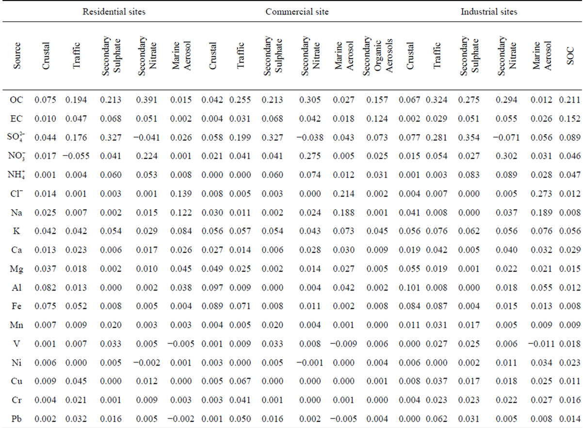
Table 7. UNMIX source composition (mass fraction) for PM2.5 sampling sites.
the region. The profiles related to high loadings of OC and EC with small loadings of metallic species indicate the impact of motor vehicle emissions because the OC/EC ratio is about 2.5 - 3.3 for gasoline exhaust, while it is 0.3 - 0.5 in diesel emissions for PM2.5 [33,34]. The ratio of OC/EC in UNMIX in this source was 3.15.
A different source associated with OC, EC,  and K was obtained by the Unmix model. This factor was associated with heavy oil combustion and biomass burning. The other new factor, that includes OC and
 , could be associated to the contribution of secondary nitrate. In the commercial and industrial sites, the principal difference with PCA was that the secondary aerosol was divided in two new sources: secondary sulfate and nitrate. It may be due to the secondary sulfate and secondary nitrate have opposing seasonal patterns, as high temperatures can accelerate sulfate formation and render secondary nitrates unstable [29].
3.4. Source Identification with PMF
The principal differences between PCA, UNMIX and PMF were found in the industrial site. A total of seven factors were chosen as the optimal number for the PMF model. These factors along with the chemical profiles (Figure 3) were associated to different sources. The first source was characterized with large amount of Cl−, Na+ and Mg, signature of fresh sea. The second source has large contributions from Al, Ca, Fe and K, mostly likely related to crustal material. The third source was identified as vehicle exhaust based upon the abundances of EC, OC and certain amount of Fe. The fourth source was related with the industrial due to the contribution of OC, Al, Cu, Cr and Pb. The next source includes OC and , could be associated to the contribution of secondary nitrate. The secondary sulphate source was recognized due to the large contribution of OC and sulphate. The last source was the heavy fuels combustion, where OC, EC, V and Ni showed an important contribution. The 83% of the experimental PM2.5 was explained according to this model.
Before estimating the source contributions, the performance of PCA/APCS, PMF and the UNMIX models were evaluated. The comparison of these three receptor models was performed by considering the following as
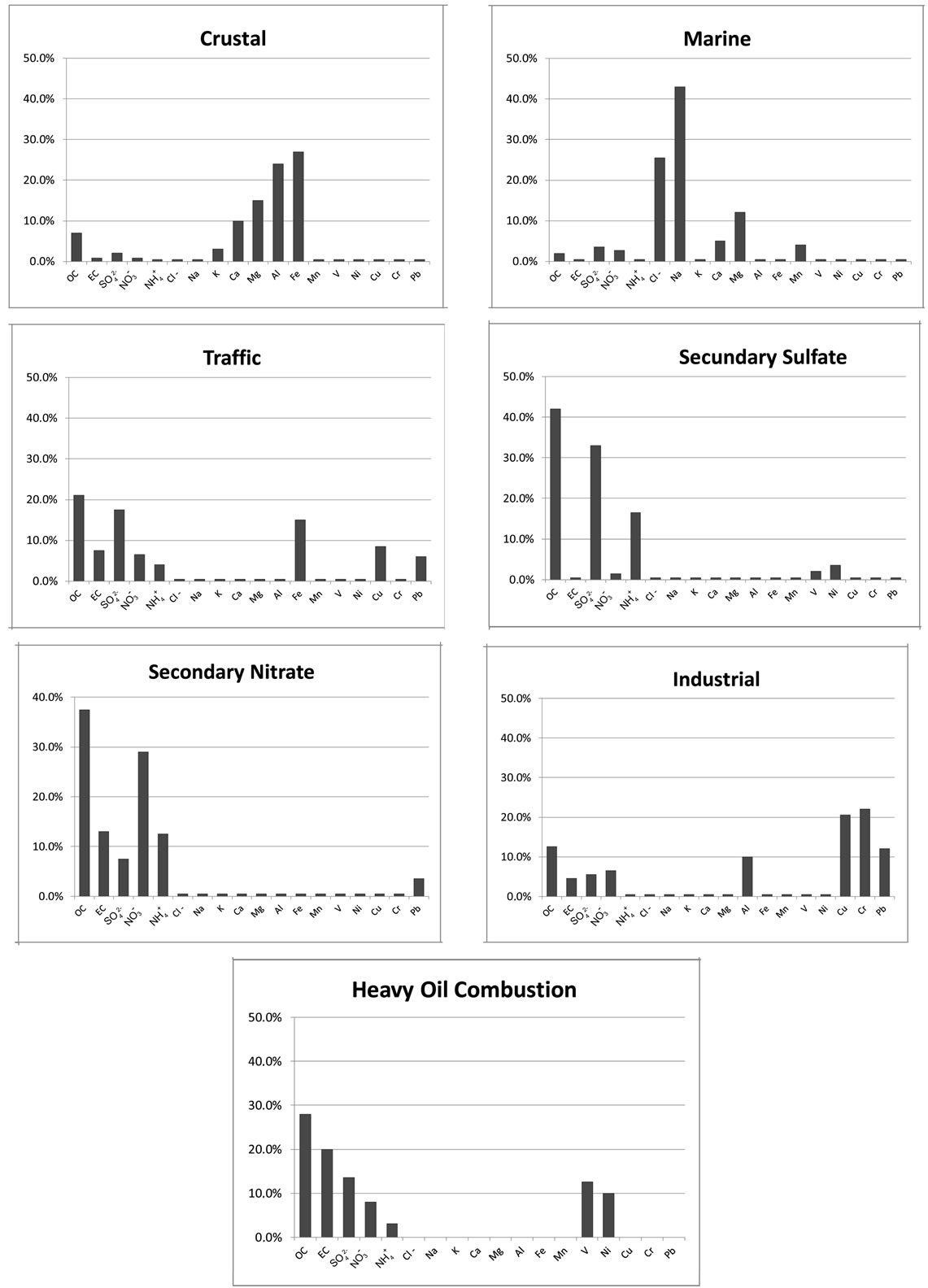
Figure 3. Percentage EV for the sources derived by PMF in an industrial site.
pects: the fitting quality between the measured PM2.5 and the predicted ones, the number and nature of the identified sources. The quality of the models was shown by regressing the predicted PM2.5 for each model against the one measured. It was found that all three models provided good results regarding their ability to reproduce measured PM2.5 concentrations with very similar slopes in all cases, being the PCA model the one with the best correlation and the closest slope to the unity. The intercepts were also similar with the lowest one for the PCA model (Table 8). However, if the calculated values by receptor models were compared with the measured concentrations for each individual chemical species, the higher mean differences were found in OC (19%),  (−17%) and
  (13%) concentrations. This situation can be explained by the fact that these species have an important contribution of secondary products that maybe weren’t well predicted by the receptor models.
An inter-comparison was also performed between the models. Good correlations were found between the three models, in particular PCA-UNMIX (r2 = 0.91, slope = 1.103) and PMF-UNMIX (r2 = 0.87, slope = 0.975).

Table 8. Lineal regression equations between PM2.5 measured values and the predicted by the receptor models in the Metropolitan Area of Costa Rica.
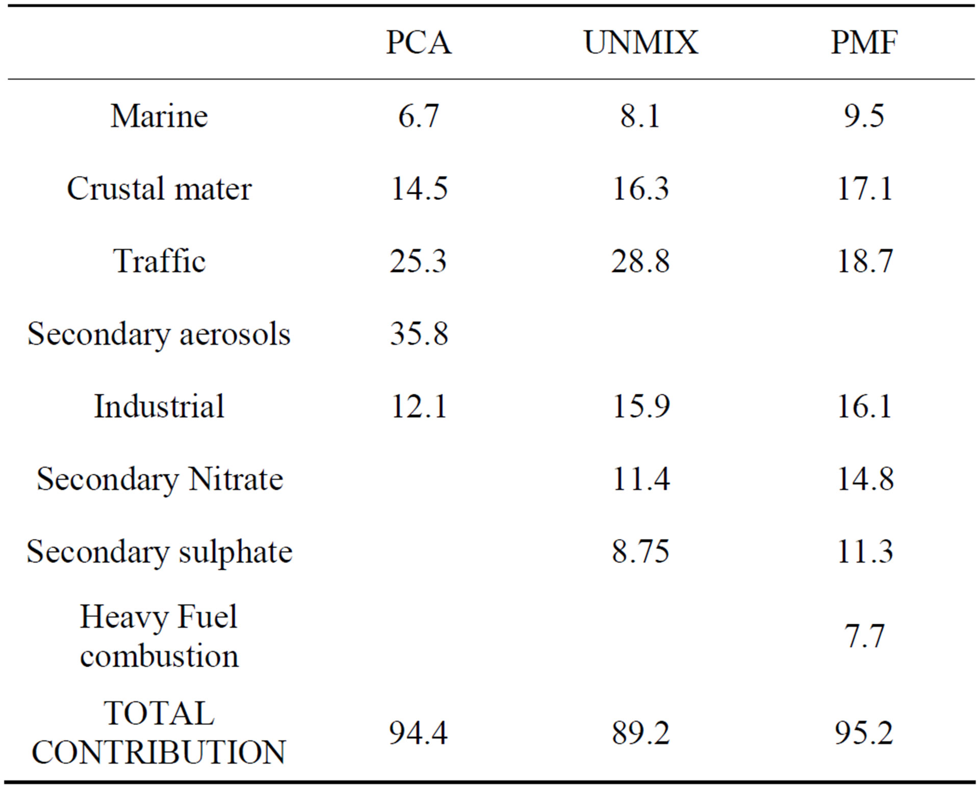
Table 9. Sources contributions (%) estimated by the three receptor models for the industrial sampling site.
3.5. Source Contributions
The contribution of each source in the different receptor models was estimated by regression analysis. The source contributions from PCA/APCS, UNMIX and PMF results for the industrial site (BE-02) are shown in Table 9.
The sum of secondary sulfate and secondary nitrate determined by UNMIX and PMF was 20.1% and 26.1%, respectively, and the secondary products apportioned by PCA was 35.8%. The secondary sulfate and secondary nitrate were not separated by PCA although they usually have opposing seasonal patterns.
PCA extracted a level of 25% from motor vehicle contributions, close to the UNMIX results (28%). PMF appointed a lower contribution to motor vehicle contribution. The vehicles also emit an important amount of NOx and VOCs, which could be transferred to secondary nitrate and secondary organic carbon (SOC) by photochemical reactions. If such particles were considered, the total contributions from motor vehicles to PM2.5 could be much higher.
PCA and UNMIX appointed industry contributions of 12.1% and 15.9%, respectively, in comparison with the 23.8% found by the PMF model. PMF model divided the industrial contribution in two factors: heavy fuels combustion and industrial. This last source included biomass burning.
In total, the PCA and PMF methods resolved 94% and 95% of the PM2.5 mass concentrations, respectively. UNMIX resolved about 89%.
4. Conclusions
The particulate matter with aerodynamic diameter less than 2.5 mm was apportioned using three multivariate receptor models: PCA-APCS, UNMIX and PMF. The present results confirmed that secondary aerosols and motor vehicles emissions were dominant mass contributors to PM2.5 in the Metropolitan Area of Costa Rica. While UNMIX and PMF were more specific in the source identification with six and seven different factors in the industrial site, respectively, PCA was more conservative and some sources could not be differentiated. It was found that all three models provided good results regarding their ability to reproduce measured PM2.5 concentrations with very similar slopes in all cases but with the PCA model showing the best correlation and the closest slope to the unity. A reasonable agreement between PMF and UNMIX was found, with both models identifying the same sources and with good correlations for the same identified sources.
This work preliminarily suggests the need to set a reference standard for PM2.5 in Costa Rica, since it only exists for PM10. Further research is needed to establish a recommendation for a PM2.5 standard in Costa Rica, since there is no sufficient data about the hourly profiles. Automatic equipment is required for this task and will be included in future work.
The important contribution of mobile and stationary combustion sources could be a short-term feasible way for the government to find control part of the PM2.5.
5. Acknowledgements
Authors would like to thank the collaboration provided by both, Environmental and Health Secretary of Costa Rica. This study is part of a Binational Cooperation Project developed by the National University in Costa Rica and the National Ecology Institute in Mexico.
REFERENCES
- F. Raes, R. Van Dingenen, E. Vignati, J.Wilson, J. P. Putaud, J. H. Seinfeld and P. Adams, “Formation and Cycling of Aerosols in the Global Troposphere,” Atmospheric Environment, Vol. 34, No. 25, 2000, pp. 4215- 4240. http://dx.doi.org/10.1016/S1352-2310(00)00239-9
- C. Arden Pope III, R. T. Burnett, M. J. Thun, E. E. Calle, D. Krewski, K. Ito and G. G. Thurston, “Lung Cancer, Cardiopulmonary Mortality, and Long-Term Exposure to Fine Particulate Air Pollution,” Journal of American Medical Association, Vol. 287, No. 9, 2002, pp. 1132-1141. http://dx.doi.org/10.1001/jama.287.9.1132
- J. Schwartz, “What Are People Dying of on High Air Pollution Days?” Environmental Research, Vol. 64, No. 1, 2002, pp. 26-35. http://dx.doi.org/10.1006/enrs.1994.1004
- G. Wang, H. Wang, Y. Yu, S. Gao, J. Feng, S. Gao and L. Wang, “Chemical Characterization of Water-Soluble Components of PM10 and PM2.5 Atmospheric Aerosols in Five Locations of Nanjing, China,” Atmospheric Environment, Vol. 37, No. 21, 2003, pp. 2893-2903. http://dx.doi.org/10.1016/S1352-2310(03)00271-1
- M. T. Cheng, Y. C. Lin, C. P. Chio, C. F. Wang and C. Y. Kuo, “Characteristics of Aerosols Collected in Central Taiwan during Asian Dust Event in Spring 2000,” Chemosphere, Vol. 61, No. 10, 2005, pp. 1439-1450. http://dx.doi.org/10.1016/j.chemosphere.2005.04.120
- J. Yin and R. M. Harrison, “Pragmatic Mass Closure Study for PM1, PM2.5 and PM10 at Roadside, Urban Background and Rural Sites,” Atmospheric Environment, Vol. 42, No. 5, 2008, pp. 980-988. http://dx.doi.org/10.1016/j.atmosenv.2007.10.005
- J. P. Putaud, R. Van Dingenen, A. Alastuey, H. Bauer, W. Birmili, J. Cyrys, H. Flentje, S. Fuzzi, R. Gehrig, H. C. Hansson, R. M. Harrison, H. Herrmann, R. Hitzenberger, C. Hüglin, A. M. Jones, A. Kasper-Giebl, G. Kiss, A. Kousa, T. A. J. Kuhlbusch, G. Löschau, W. Maenhaut, A. Molnar, T. Moreno, J. Pekkanen, C. Perrino, M. Pitz, H. Pusbaum, X. Querol, S. Rodriguez, I. Salma, J. Schwarz, J. Smolik, J. Scheneider, G. Spindler, H. Ten Brink, J. Tursic, M. Viana, A.Wiedensohler and F. Raes, “A European Aerosol Phenomenology-3: Physical and Chemical Characteristics of Particulate Matter from 60 Rural, Urban, and Kerbside Sites across Europe,” Atmospheric Environment, Vol. 44, No. 10, 2010, pp. 1308-1320. http://dx.doi.org/10.1016/j.atmosenv.2009.12.011
- J. G. Watson, T. Zhu, J. C. Chow, J. Engelbrecht, E. M. Fujita and W. E. Wilson, “Receptor Modeling Application Framework for Particle Source Apportionment,” Chemosphere, Vol. 49, No. 9, 2002, pp. 1093-1136. http://dx.doi.org/10.1016/S0045-6535(02)00243-6
- J. G. Watson, L. Chen, J. C. Chow, D. H. Lowenthal and P. Doraiswamy, “Source Apportionment: Findings from the US Supersite Program,” Journal of the Air & Waste Management Association, Vol. 58, No. 2, 2008, pp. 265- 288. http://dx.doi.org/10.3155/1047-3289.58.2.265
- J. Watson and J. Chow, “Receptor Models for Air Quality Management,” EM, 2004, pp. 15-24.
- IUPAC, “Compendium of Chemical Terminology, 2nd Ed (the ‘Gold Book’),” Compiled by A. D. McNaught and A. Wilkinson, Blackwell Scientific Publications, Oxford, 1997.
- S. Marcazzan, G. Vaccaro and R. Vecchi, “Characterisation of PM10 and PM2.5 Particulate Matter in the Ambient air of Milan (Italy),” Atmospheric Environment, Vol. 35, No. 27, 2001, pp. 4639-4650. http://dx.doi.org/10.1016/S1352-2310(01)00124-8
- J. Herrera, “Costa Rica Metropolitan Area Emission Inventory 2007,” National University, Costa Rica, 2009, pp. 460-489.
- P. K. Hopke, “Receptor Modeling for Air Quality Management,” In: B. G. M. Vandeginste and O. M. Kvalheim, Eds., Data Handling in Science and Technology, Elsevier, Amsterdam, 1991.
- R. Henry, “UNMIX Version 2.4 Manual,” US Environmental Protection Agency, Research Triangle Park, 2001.
- R. L. Poirot, P. R. Wishinski, P. K. Hopke and A. V. Polissar, “Comparative Application of Multiple Receptor Methods to Identify Aerosol Sources in Northern Vermont,” Environmental Science and Technology, Vol. 35, No. 23, 2001, pp. 4622-4636. http://dx.doi.org/10.1021/es010588p
- L. W. A. Chen, B. G. Doddridge, R. R. Dickerson, J. C. Chow and R. C. Henry, “Origins of Fine Aerosol Mass in the Baltimore-Washington Corridor: Implications from Observation, Factor Analysis, and Ensemble Air Parcel Back Trajectories,” Atmospheric Environment, Vol. 36, No. 28, 2002, pp. 4541-4554. http://dx.doi.org/10.1016/S1352-2310(02)00399-0
- H. Hellen, H. Hakola and T. Laurila, “Determination of Source Contribution of NMHC in Helsinki (60˚N, 25˚E) Using Chemical Mass Balance and the UNMIX Multivariate Receptor Models,” Atmospheric Environment, Vol. 37, No. 11, 2003, pp. 1413-1424. http://dx.doi.org/10.1016/S1352-2310(02)01049-X
- P. Paatero, “Least Square Formulation of Robust NonNegative Factor Analysis,” Chemometrics and Intelligent Laboratory, Vol. 37, No. 1, 1997, pp. 23-35. http://dx.doi.org/10.1016/S0169-7439(96)00044-5
- P. D. Hien, V. T. Bac and N. T. H. Thinh, “PMF Receptor Modelling of Fine and Coarse PM10 in Air Masses Governing Monsoon Conditions in Hanoi, Northern Vietnam,” Atmospheric Environment, Vol. 38, No. 2, 2004, pp. 189-201. http://dx.doi.org/10.1016/j.atmosenv.2003.09.064
- E. Kim, T. V. Larson, P. K. Hopke, C. Slaughter, L. E. Sheppard and C. Claiborn, “Source Identification of PM2.5 in an Arid Northwest US City by Positive Matrix Factorization,” Atmospheric Research, Vol. 66, No. 4, 2003, pp. 291-305. http://dx.doi.org/10.1016/S0169-8095(03)00025-5
- F. Mazzei, A. Alessandro, F. Lucarelli, S. Nava, P. Prati, G. Valli and R. Vecchi, “Chracterization of Particulate Matter Sources in an Urban Environment,” Science of Total Environment, Vol. 401, No. 1-3, 2008, pp. 81-89. http://dx.doi.org/10.1016/j.scitotenv.2008.03.008
- P. Paatero and P. K. Hopke, “Discarding or Downweighting High-Noise Variables in Factor Analytic Models,” Analytical Chimica Acta. Vol. 490, No. 1-2, 2003, pp. 277-289. http://dx.doi.org/10.1016/S0003-2670(02)01643-4
- P. Paatero, “User’s Guide for Positive Matrix Factorization Programs PMF2 and PMF3, Part 1: Tutorial,” US Environmental Protection Agency, 2000.
- L. M. Castro, C. A. Pio, R. M. Harrison and D. J. T. Smith, “Carbonaceous Aerosol in Urban and Rural European Atmospheres: Estimation of Secondary Organic Carbon Concentrations,” Atmospheric Environment, Vol. 33, No. 17, 1999, pp. 2771-2781. http://dx.doi.org/10.1016/S1352-2310(98)00331-8
- J. Herrera, J. F. Rojas, S. Rodriguez, V. H. Beita, D. Solorzano, A. Campos, B. Cardenas and D. G. Baumgardner, “Temporal and Spatial Variations in Organic and Elemental Carbon Concentrations in PM10/PM2.5 in the Metropolitan Area of Costa Rica, Central America,” Atmospheric Pollution Research, Vol. 4, 2013, pp. 53-63.
- C. Hueglin, R. Gehrig, U. Baltensperger, M. Gysel, C. Monn and H. Vonmont, “Chemical Characterisation of PM2.5, PM10 and Coarse Particles at Urban, Near-City and Rural Sites in Switzerland,” Atmospheric Environment, Vol. 39, No. 4, 2005, pp. 637-651. http://dx.doi.org/10.1016/j.atmosenv.2004.10.027
- P. Warneck, “Chemistry of the Natural Atmosphere,” Wiley and Sons, Academy Press, 1987, p. 757.
- J. Sternbeck, A. Sjödin and K. Andréasson, “Metal Emissions from Road Traffic and the Influence of Resuspension: Results from Two Tunnel Studies,” Atmospheric Environment, Vol. 36, No. 30, 2002, pp. 4735-4744. http://dx.doi.org/10.1016/S1352-2310(02)00561-7
- J. H. Seinfeld and S. N. Pandis, “Atmospheric Chemistry and Physics from Air Pollution to Climate Change,” Wiley, New York, 1998, pp. 649-655.
- J. P. Putaud, F. Raes, R. Van Dingenen, E. Brüggemann, M. C. Facchini, S. Decesari, S. Fuzzi, R. Gehrig, C. Hüglin, P. Laj, G. Lorbeer, W. Maenhaut, N. Mihalopoulos, K. Müller, X. Querol and S. Rodriguez, “A European Aerosol Phenomenology-2: Chemical Characteristics of Particulate Matter at Kerbside, Urban, Rural and Background Sites in Europe,” Atmospheric Environment, Vol. 38, 2004, pp. 2579-2595.
- M. Zheng, L. G. Salmon, J. J. Schauer, L. Zeng, C. S. Kiang and Y. Zhang, “Seasonal Trends in PM2.5 Source Contributions in Beijing, China,” Atmospheric Environment, Vol. 39, No. 22, 2005, pp. 3967-3976. http://dx.doi.org/10.1016/j.atmosenv.2005.03.036
- F. K. Duan, K. B. He, F. M. Yang, X. C. Yu, S. H. Cadle and T. Chan, “Concentrations and Chemical Characteristics of PM2.5 in Beijing, China: 2001-2002,” Science of Total Environment, Vol. 355, No. 1-3, 2006, pp. 264-275. http://dx.doi.org/10.1016/j.scitotenv.2005.03.001
- S. H. Cadle, P. A. Mulawa, E. C. Hunsanger, K. E. Nelson, R. A. Ragazzi and R. Barrett, “Composition of LightDuty Motor Vehicle Exhaust Particulate Matter in the Denver, Colorado Area,” Environmental Science and Technology, Vol. 33, No. 14, 1999, pp. 2328-2339. http://dx.doi.org/10.1021/es9810843
NOTES
*Corresponding author.