ABSTRACT

Redistributions of income can be considered as variable transformations of the initial income variable. The transformation is usually assumed to be positive, monotone-increasing and continuous, but discontinuous transformations have also been discussed recently. If the transformation is a tax or a transfer policy, the transformed variable is either the post-tax or the post-transfer income. A central problem has been the Lorenz dominance between the initial and the transformed income. This study considers analyses of other properties of the transformed Lorenz curves, especially its limits. We take in account mainly two cases (a) the transformed variable Lorenz dominates the initial one and (b) the initial Lorenz dominates the transformed one. For applications, the first case is more important than the second. The limits obtained are not accurate for a specific transformation, but do hold generally for all distributions and a broad class of transformations so that, if one pursues general conditions the inequalities obtained cannot be improved.

1. Introduction

Redistributions of income according to tax or transfer policies can be considered as variable transformations of the initial income. The transformation is usually assumed to be positive, monotone-increasing and continuous. The initial results are given in Theorem 1. [1-3] Consider a nonnegative random variable X with the distribution function, mean and Lorenz curve. Let be a continuous monotone increasing function and assume that exists. Then Lorenz curve for exists and 1) if is monotone decreasing2) if is constant and 3) if is monotone increasing.

The importance of case (1) is that it gives the inequality effect of progressive taxation. The case (2) corresponds to flat taxes. The last case (3) is of minor economic importance, but it is included in order to complete the theorem. Recently, Fellman [4,5] has also discussed discontinuous transformations. If the transformation is considered as a tax or a transfer policy, the transformed variable is either the post-tax or the post-transfer income. Under the assumption that Theorem 1 should hold for all income distributions, the conditions are both necessary and sufficient [2,4]. Hemming and Keen [6] have given an alternative version of the conditions. In this study we consider other general properties of the transformed Lorenz curves.

2. Background

Consider income X, defined on the interval, where, with the distribution function, density function, mean, percentile defined as and Lorenz curve. The general formulae are

(1)

and

(2)

where.

We consider the transformation, where is non-negative, continuous and monotone-increasing. Since the transformation can be considered as a tax or a transfer policy, the transformed variable is either the post-tax or the posttransfer income.

The mean and the Lorenz curve for variable Y are

(3)

and

(4)

A fundamental theorem concerning Lorenz dominance is [2,4].

Theorem 2. Let be an arbitrary, non-negative, random variable with the distribution, mean and Lorenz curve. Let be a nonnegative, monotone-increasing function, let and let exist. The Lorenz curve of Y exists and the following results hold:

1) if and only if is monotone-decreasing

2) if and only if is constant and

3) if and only if is monotone-increasing.

In the following, we consider additional properties of the Lorenz curve. If

is constant, then according to Theorem 1 (2), and the transformed Lorenz curve is identical with the initial one, a case which will be ignored.

3. Results

3.1. The Ratio Is Monotonically Decreasing

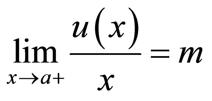
According to Theorem 1 Lorenz dominates. We introduce the values M and m such that

and

.

Consequently,

.

Let,. Assume that and that and consequently,

.

Note that points and are chosen arbitrarily and that the equality signs cannot be ignored because we also include the functions

which are not uniformly strict decreasing in the class of transformations. Hence, we have to include members for which equalities hold for almost the whole range and, in addition, sub-intervals in which strict inequalities hold can be chosen arbitrarily short and located arbitrarily within the range. If one pursues general conditions, the inequalities (8) and (9) obtained below cannot be improved. If we assume that

is monotonically decreasing, then must be continuous, otherwise

should have positive jumps [1].

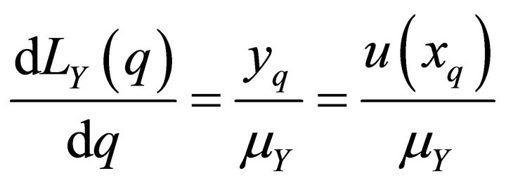
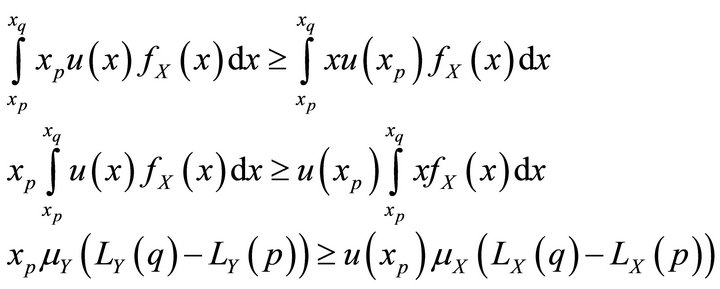
From

it follows that. The integration over the interval yields

(5)

and

.

Analogously, it follows from

that, and we obtain

. (6)

Consequently,

. (7)

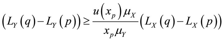
When in (7), then

and one obtains

. (8)

The lower bound gives an evaluation of how much the Lorenz curve has increased. The upper bound is of minor interest and is commented on later.

When in (7), then

and one obtains

.

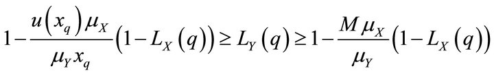
In order to compare these inequalities with the inequalities in (8), we change the argument from p to q, and the inequalities are

(9)

The lower bound gives an evaluation of how much the Lorenz curve has increased. The upper bound is of minor interest and is discussed later.

Inequality (8) is applicable to small values and inequality (9) to large values of q. For small values of q, we consider the difference

(10)

and for large q we consider the difference

. (11)

In general,

and

.

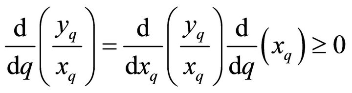
The ratio

is decreasing and consequently

.

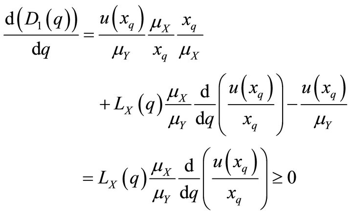
Now we differentiate and obtain

Consequently is increasing from zero at to a maximum for (say).

Now we differentiate and obtain

Consequently is decreasing from to zero when. The point, at which the shift from (10) to (11) is performed, is chosen so that. Now,

;

that is,

.

Consequently,

Since the ratio

is decreasing, the difference

shifts its sign from plus to minus at point. Hemming and Keen ([6]) gave the condition for Lorenz dominance that

crosses the

level once from above. Our results above have shown that the crossing point is. The condition obtained can also be otherwise explained. If we write it as

we obtain the formula

that is, the Lorenz curves and have parallel tangents and the distance between the Lorenz curves is maximal for.

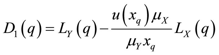
We define the difference function as

, (12)

and the lower bound of is

. (13)

Figure 1 shows the Lorenz curves, , the lower bound and the difference between and the lower bound.

Remarks. The variable Y Lorenz dominates X, and the upper bounds in (8) and (9) tells us nothing about the reductions in the inequality. The upper bound contains the maximum value and one has to take it for granted that it is also inaccurate when M is finite. In addition, there may be situations in which. The minimum value m can be zero, and in this case the upper bound is one and the obvious inequality is obtained.

3.2. The Ratio Is Monotonically Increasing

The analysis of this case follows similar traces to the earlier study and the results are analogous to our earlier results, but in this case may be discontinuous. Only the inequality signs have changed their directions. We introduce the values and such that

and

and consequently

.

Note, that in this case the points and are also chosen arbitrarily and that the equality signs cannot be ignored because we also include functions

which are not uniformly strictly increasing in the class of transformations. Hence, we have to include members for which equalities hold for almost the whole range and, in addition, the subintervals where strict inequalities hold can be arbitrarily short and can be located arbitrarily within the range. If one pursues general conditions, the inequalities (17) and (18) obtained below cannot be improved.

If is discontinuous, the discontinuities can only

be a countable number of finite positive jumps. Under such circumstances is still integrable.

We use the same notations as above and assume that, that and consequently that.

Now,

.

Consider. The integration over the interval yields

(14)

and

.

Analogously, if we consider we obtain

(15)

and

.

Hence,

. (16)

When in (16), then

and one obtains

. (17)

Now, the initial variable X Lorenz dominates the transformed Y and the upper bound is the interesting case.

When in (16), then

one obtains

After a shift from p to q, we obtain

(18)

Now the upper bound is of interest. Formula (17) is applicable for small values and formula (16) for large values of q. In the following, we consider the difference between the upper bound and the Lorenz curve, that is, for small values of q

. (19)

For large values of q, we consider the difference

. (20)

In general,

.

The ratio

is increasing and consequently,

.

Now we differentiate and note that

is increasing and obtain

.

Consequently is increasing from zero to a maximum for.

Now we differentiate and obtain

.

Consequently is decreasing from a maximum to zero. The point denoted, at which the shift from to is performed, satisfies .

Now,

that is,

.

This condition is identical with the condition, given above, in which

is decreasing.

Again, the condition

can be written

and we obtain the formula

that is, the Lorenz curves and have parallel tangents and the distance between the Lorenz curves is maximal.

We define the difference function as

, (21)

and the upper bound of is

(22)

In Figure 2, we sketch the Lorenz curves, , the upper bound and the difference between the upper bound and.

Now the lower bounds are of minor interest because the initial variable X Lorenz dominates Y. Note that is possible in some situations and the lower bound in (17) can be zero. Note that M can be great and even is possible in some situations and the lower bound in (18) can be even negative.

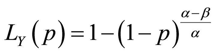
Example 1. The Pareto distribution. Consider income X with the Pareto distribution and, where and. Now,

and the Lorenz curve

.

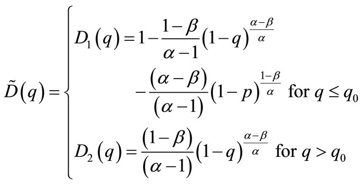
From we obtain. Let the transformation be so that the function is decreasing. We obtain, the Lorenz curve

,

and

For, the ratio

is decreasing, this case being sketched in Figure 1, and if the ratio

is increasing, this case being sketched in Figure 2.

4. Conclusion

Redistributions of income have commonly been defined as variable transformations of the initial income variable. The transformations are mainly considered as tax or transfer policies yielding post-tax or post-transfer incomes and therefore, the transformations are usually assumed to be positive, monotone-increasing and continuous. Recently, discontinuous transformations have also been discussed. The fundamental concern has been the Lorenz ordering between the initial and the transformed income. In this study we constructed limits for he transformed Lorenz curves. We considered the optimal cases that the transformed variable Lorenz dominates the initial one and the initial variable Lorenz dominates the transformed one. In applications, the first case is more important than the second, because it yields policies which reduce the inequality. The case (2) in Theorem 2 is not included in this study because the initial and the transformed Lorenz curves are identical. The limits obtained hold generally for all distributions and a broad class of transformations. If one pursues general conditions the inequalities obtained cannot be improved.

5. Acknowledgements

We are grateful to an anonymous referee for comments and suggestions on a previous version of the manuscript. This study was in part supported by a grant from the “Magnus Ehrnrooths Stiftelse” Foundation.

REFERENCES

- J. Fellman, “The Effect of Transformations on Lorenz Curves,” Econometrica, Vol. 44, No. 4, 1976, pp. 823- 824. doi:10.2307/1913450
- U. Jakobsson, “On the Measurement of the Degree of Progression,” Journal of Public Economics, Vol. 5, No. 1-2, 1976, pp. 161-169. doi:10.1016/0047-2727(76)90066-9
- N. C. Kakwani, “Applications of Lorenz Curves in Economic Analysis,” Econometrica, Vol. 45, No. 3, 1977, pp. 719-727. doi:10.2307/1911684
- J. Fellman, “Discontinuous Transformations, Lorenz Curves and Transfer Policies,” Social Choice and Welfare, Vol. 33, No. 2, 2009, pp. 335-342. doi:10.1007/s00355-008-0362-4
- J. Fellman, “Discontinuous Transfer Policies with Given Lorenz Curve,” Advances and Applications in Statistics, Vol. 20, No. 2, 2011, pp. 133-141.
- R. Hemming and M. J. Keen, “Single Crossing Conditions in Comparisons of Tax Progressivity,” Journal of Public Economics, Vol. 20, No. 3, 1993, pp. 373-390. doi:10.1016/0047-2727(83)90032-4