ABSTRACT

Under the constraint that the initial capital is not enough for a perfect hedge, the problem of deriving an optimal partial hedging portfolio so as to minimize the shortfall risk is worked out by solving two connected subproblems sequentially. One subproblem is to find the optimal terminal wealth that minimizes the shortfall risk. The shortfall risk is quantified by a general convex risk measure to accommodate different levels of risk tolerance. A convex duality approach is used to obtain an explicit formula for the optimal terminal wealth. The second subproblem is to derive the explicit expression for the admissible replicating portfolio that generates the optimal terminal wealth. We show by examples that to solve the second subproblem, the Malliavin calculus approach outperforms the traditional delta-hedging approach even for the simplest claim. Explicit worked-out examples include a European call option and a standard lookback put option.

1. Introduction

A replicating (self-financing) portfolio designed to eliminate the risk exposure of the target contingent claim completely is called a perfect hedge. Since the value of a perfect hedging portfolio achieves exact replication of the payoff of the target security at the expiration date T, one can offset the risk of the target claim by selling the replicating strategy. In a financial market that is complete and arbitrage free, a perfect hedging strategy exists for any contingent claim with a sufficiently integral terminal payoff. The cost of replication is given by the expected value of the discounted payoff under the unique, risk neutral equivalent martingale measure, i.e.,

(1)

where is the price of the risk-free asset.

One of the drawbacks of a perfect hedge is that the initial cost of the exact replication (i.e., in (1)) is high. In addition, avoiding risks completely means losing out on the potential gain that accepting the risk may have allowed. To this end, we discuss the position of an agent who is unwilling to commit at time the entire amount necessary for implementing a perfect hedge and is thus interested in a partial hedging strategy that offers the balance between the cost and the risk exposure. Our goal is to derive optimal partial hedging strategies for various target contingent claims.

Since the shortfall risk is intrinsic in a partial hedging environment, one natural way to find the optimal partial hedging strategy would be to minimize the shortfall risk under the constraint that the initial capital is less than (i.e., the amount required for a perfect hedge). The criterion used to quantify the shortfall risk is the expectation of the shortfall weighed by a convex loss function g, where is the terminal payoff of a target contingent claim and is the value of the hedging portfolio. Compared with the linear loss function criterion adopted by [1] and [2], convexity of the loss function g offers the flexibility to accommodate different types of market participants with different levels of risk tolerance. For example, pension funds and foundations are usually risk-averse whereas hedge funds are more likely to have risk-seeking behaveiors. Moreover, individual investors’ attitudes towards risk are unique depending on their own personal and financial circumstances.

The problem of solving for an optimal partial hedging portfolio so as to minimize the shortfall risk is decomposed into two subproblems. One subproblem is to find the attainable terminal wealth that minimizes the shortfall risk under the insufficient initial capital constraint. A convex duality approach is used to obtain an explicit formula for the optimal terminal wealth. We are the first to use the convex duality approach to study this problem in a systematic way for a general convex loss function. A similar problem was solved in [3] applying the Neyman Pearson lemma. The second subproblem is to derive the explicit expression for the admissible replicating portfolio that generates the optimal terminal wealth. There are two different approaches to solving the second subproblem. One is the well-known delta-hedging approach and the other is the Malliavin calculus approach. [4] compared these two approaches in the Black and Scholes environment. The author commented that the difficulty of applying the delta-hedging approach is to verify the continuous differentiability condition of the price process of the target claim. In the case of perfect hedge, the difficulty noted above does not exist for a standard call option. The Malliavin calculus approach is only needed for certain path dependent options such as lookback options. However, this is no longer the case in the partial hedging environment. We find that to derive an optimal partial hedging portfolio even for the simplest claim such as an ordinary call option, it is not trivial to verify the continuous differentiability condition for the price process of the optimal terminal wealth. Nevertheless the machinery of the Malliavin calculus approach help circumvent this difficulty. Although the full range of cases remain to be investigated, we illustrate by examples that in the context of partial hedging, the Malliavin calculus approach is not only mathematically rigorous, but also straightforward and easy to implement. Explicit worked-out examples in previous partial hedging studies are only restricted to standard European options. In this paper, by applying the Malliavin calculus approach, we are able to obtain the explicit partial hedging formula for a lookback option.

It is worth noting that the Malliavin calculus approach has gained considerable interest since it was first introduced to the portfolio theory literature by [5]. For example, [6] applied the Clark-Ocone formula and the gradient operator in Malliavin calculus to derive an explicit representation for the optimal trading strategy in the case of partial information. The Malliavin calculus approach has also been used to derive perfect hedging strategies for lookback and barrier options (see [7,8]). [9] found the Malliavin calculus approach useful in deriving the hedging portfolios for an expected-utility-maximizing investor whose consumption rate and terminal wealth are subject to downside constraints.

The rest of the paper is organized as follows. Section 2 sets up the model for the financial market, presents the dynamics of the agent’s wealth process, and defines the class of admissible portfolios. Section 3 solves the problem of minimizing the expected shortfall loss using the convex duality approach. The main result is an explicit expression for the optimal terminal wealth. The existence of an optimal hedging strategy is shown as well. The Malliavin calculus approach is summarized in Section 4 and is used to derive the optimal partial hedging portfolios for two specific examples in Section 5.

2. The Economy

Since our ultimate interest is to obtain explicit expressions for the optimal partial hedging portfolios, the model under consideration here is a typical Black and Scholes economy as in [10], wherein there are one riskless asset of price and one risky asset of price. We shall assume that the riskless asset earns a constant instantaneous rate of interest, and that the price of the risky asset follows a geometric Brownian motion. More specifically, the respective prices and evolve according to the (stochastic) differential equations

(2)

(3)

All our problems are treated on a finite time-horizon [0,T]. In Equation (3), is a standard Brownian motion on a complete probability space endowed with an augmented filtration generated by the Brownian motion. We assume that (interest rate), (stock return rate), (stock volatility), and are positive constants.

Set “the market-price-of-risk”. We introduce the following processes

(4)

(5)

and the auxiliary probability measure defined on

(6)

According to the Girsanov theorem the process is a -Brownian motion on.

In the context of the above market model, consider an agent who is endowed with initial wealth, can decide, at each time, which amount to invest in the risky asset without affecting its price. We shall denote by the wealth of this agent at time. With chosen, the investor places the amount in the bank account. The agent’s wealth process satisfies the equation

(7)

Formally, we say that a trading strategy over the time interval is self-financing if its wealth process satisfies (7). We require that the wealth process in (7) to be almost surely uniformly bounded from below by zero for the trading strategies to be admissible. The class of all such admissible trading strategies is denoted by. Let us introduce the notation

(8)

the discounted version of the wealth process. We have the equivalent equation

(9)

We can deduce that the discounted wealth process is a continuous local martingale under. Denoting the process

(10)

with the help of the “Bayes rule”, we can deduce that the process is a continuous local martingale under. This process is also bounded from below. An application of Fatou’s lemma shows that is a supermartingale under. Consequently, we have

(11)

Moreover, it is well-known that this market is complete in the following sense: for every initial wealth such that and every nonnegative random variable, there exists an admissible trading strategy whose value process satisfies , P-almost surely.

3. Minimizing the Expected Shortfall Risk

This section is devoted to finding an explicit expression of the optimal terminal wealth that minimizes the expected shortfall risk. Consider a contingent claim whose terminal payoff is given by a -measurable, nonnegative random variable C. Recall defined in (1) and assume. The value is the smallest amount such that there exists an admissible strategy whose value process satisfies, P-almost surely (i.e., a perfect hedge). Notice that the notations and are interchangeable. In this section, we choose to use the latter to emphasize the value of the portfolio is achieved by a certain amount of initial capital and a specific admissible strategy.

Now assume that the initial capital is not enough to do a perfect hedge, i.e.,. The risk measure used to find the optimal partial hedging strategy takes account of two factors. One is the size of the shortfall, where. The other is the investor’s attitude towards the shortfall risk, which is captured by a loss function. We assume that is an increasing and strictly convex function defined on, with. We further assume that is in, , and

(12)

We now give the formal definition of the risk measure.

Definition 3.1 The shortfall risk is defined as the expectation

(13)

of the shortfall weighed by the loss function.

Remark 3.1 A special case of the risk measure defined above is the lower partial moment (e.g., [11]) with, for some.

Our aim is to find an admissible portfolio which solves the optimization problem

(14)

for any.

This stochastic control problem is solved by first finding the optimal terminal wealth that mini mizes the shortfall risk in (13) under the constraint that. We first make the following useful observation.

Lemma 3.1 Let such that

. Then there exists a such that

The proof of the lemma is deferred to the Appendix. In view of Lemma 3.1, we can (and do) assume that P-almost surely in (14). Hence the risk measure can be written as. As noted earlier, is assumed to be nonnegative. Hence for any admissible portfolio strategy, we have. Define as the inverse of. In the case of, we can extend the domain of to by letting for. We shall adopt useful tools from convex duality: starting with the function, consider its (random, -measurable) Legendre transform

(15)

(16)

The supremum is attained by

(17)

For the convenience of the reader, we summarize below some basic properties of the function.

Lemma 3.2 The function enjoys the following properties.

1) for all. is nondecreasing on.

2) The function is convex and continuous.

Proof. a) It follows from the explicit expression of in (16) that is nondecreasing. From the facts that is nondecreasing and for, it is easy to see that for all.

b) We see immediately from (15) that is a convex function, since it is the pointwise supremum of a family of convex (indeed, affine) functions of. Note that this is true whether or not is convex. is continuous on since a convex function is continuous on an open interval. Continuity of at follows directly from the explicit expression of in (16).

It follows that for any initial capital

, we have

(18)

almost surely. Thus, in conjunction with (6) and (11), we obtain

(19)

where we set

(20)

(21)

Now assume that for every, we have

(22)

Remark 3.2 Note that (22) is not assumed for. So the above assumption still allows, which is the case for many popular options.

The function in (20) possesses the following useful property.

Lemma 3.3 Assume that satisfies (22). The function in (20) is continuous on.

Proof. First we show that the function

is continuous. Let be a sequence of non-negative numbers converging to. If, then by assumption (22),

almost surely. Hence and the dominated convergence theorem implies the continuity of. Assume now that. Then one can see by separating the cases and that

almost surely. Another application of the dominated convergence theorem implies that is continuous even at. The continuity of

follows similarly using the bound

and the dominated convergence theorem.

To derive the maximum of in (19), we assume that is in and

(23)

From (16) it follows that is convex and continuous on, and continuously differentiable on.

In particular,

(24)

For every, we have

(25)

Indeed, by assumption (23),

(26)

We now establish the following auxiliary result.

Lemma 3.4 Define. Then is convex on, continuously differentiable on, and

(27)

Proof. Convexity of is inherited from. For any, let be an arbitrary positive number such that belongs to. Then

as, almost surely, and by the convexity of for

Relation (25) and the dominated convergence theorem imply

(28)

The right hand side of (28) is exactly by (24) and (20). We know from Lemma 3.3 that is continuous. So is indeed continuously differentiable.

Now we have. The function is concave on, belongs to, and satisfies. Note also that

and

So achieves its maximum over at

(29)

Therefore, (19) gives

(30)

The following is the crucial observation in the duality approach.

Remark 3.3 (Sufficient and necessary conditions for strong duality) The inequality of (19) holds as equality for some and with, if and only if we have

(31)

and

(32)

Now we are ready to state the main result of this section.

Proposition 3.1 For every, the value is given by (29) and the -measurable random variable

(33)

satisfies

(34)

Proof. From (20), (1), and the fact that

we see that

Remark 3.4 Notice that whenever, the optimal terminal wealth in (33) has a simple form of

. A typical example is the case of lower partial moment with, for some.

For the sake of completeness, we include an existence result of the optimal hedging strategy.

Theorem 3.1 Existence of optimal strategy. For any given, and with given by (29) and given by (33), there exists a portfolio process for which (31) and (32) hold and which is optimal for the problem of (14):

(35)

In particular, it is equal to that portfolio which replicates the claim of (33).

Proof. From Proposition 3.1, we can find an - measurable random variable such that (34) holds. Consider now the -martingale (in the notation of (33))

(36)

written in its representation as a stochastic integral with respect to for a suitable portfolio process (see [12], p. 93). The process satisfies and the requirement that it’s bounded from below by zero, so. The optimality of is then a consequence of Remark 3.3.

4. The Malliavin Calculus Approach

To solve the second subproblem of deriving the partial hedging portfolios that generate the optimal terminal wealth in (33), we consider two different approaches. One is the well-known -hedging approach and the other is the Malliavin calculus approach. For easy reference and to make the paper self-contained, we first briefly recap the concept of -hedging. Then we introduce the definition of the Mallivin derivative of a random variable and the Clark-Ocone formula. Thereafter, we present a Mallivin calculus approach for deriving the replicating portfolio as first used in [5].

In the standard Black and Scholes framework, the -hedging approach works in the following way. In a complete financial market, the optimal wealth process (The notations and are used interchangeably.) is given by the discounted conditional expectation of the optimal terminal wealth under the risk neutral probability measure, i.e.,. In many situations, the optimal wealth process is a Markov process and is in the form of, where is the time t stock price. If the condition that is a -function is verifiable, we can apply the Itô formula to to obtain

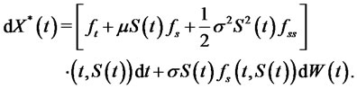(37)

The replicating portfolio is denoted by

where denotes the number of units to be held at time in the risk-free asset, and denotes the number of units to be held in the stock at time. Notice the relationship between and given by. By the definition of a self-financing portfolio, we have

(38)

From the uniqueness of the Itô integral it follows that we can use (37) and (38) to identify the replicating portfolio, where

(39)

(40)

Equation (40) is the famous -hedging formula. As pointed out in [4], the major difficulty of using the -hedging approach is to verifty satisfies the necessary differentiability condition. We show by examples in the next section how the Malliavin calculus approach can help us get around this difficulty in the partial hedging context.

The main components for the Malliavin calculus approach to work are the gradient operator and the ClarkOcone formula. Let denote the family of all random variables of the form

where is a polynomial in variables and for some

(deterministic). Notice that the set is dense in. Next, we define the Cameron-Martin space according to

and identify our probability space with

such that for all. Here denotes the Wiener space—the space of all continuous, real-valued functions on such that, denotes the corresponding Borel -algebra, and denotes the unique Wiener measure. With this setup we can define the directional derivative of a random variable in all the directions by

(41)

Notice from the above equation that the map is continuous for all and linear, consequently there exists a stochastic variable with values in the Cameron-Martin space such that

.

Moreover, since is an -valued stochastic variable, the map is absolutely continuous with respect to the Lebesgue measure on. Now we let the Malliavin derivative denote the Radon-Nikodym derivative of with respect to the Lebesgue measure such that

(42)

If we define this expression with Equation (41) we have the following result, which in many cases is taken directly as a definition.

Definition 4.1 The Malliavin derivative of a stochastic variable is the stochastic process

given by

We note that the Malliavin derivative is well defined almost everywhere.

Let us introduce a norm on the set according to

(43)

Now, as the Malliavin derivative is a closable operator (see [13]), we define by the Banach space which is the closure of under the norm.

The Clark-Ocone formula is the cornerstone of the Malliavin calculus hedging approach. This formula is a generalization of the Itô representation theorem (see [14]) in the sense that it gives an explicit expression for the integrand. The original Clark-Ocone formula (see [13]) applies to any -measurable stochastic variable in the space.

[8] shows that the Clark-Ocone formula is valid for any -measurable stochastic variable in and therefore the Malliavin calculus approach to deriving the replicating portfolio of a contingent claim as in [5] can be extended in a similar way. However, since all of the examples discussed later in the paper only use the Clark-Ocone formula to the stochastic variables in, we only state the original Clark-Ocone formula in [13] and the results in [5] as a theorem. We refer the interested readers to [8] for the extensions.

Theorem 4.1 Let the stochastic variable belong to. Then we have the representation formula

Following the above Clark-Ocone formula and the results in [5], any optimal portfolio can be replicated by the self-financing portfolio

(44)

In order to derive the replicating portfolio using the above theorem, we need to calculate the Malliavin derivative of. When is a Lipschitz function of a stochastic vector process belonging to, the following classic chain rule as proved in [13] can be used to calculate.

Proposition 4.1 (Classic Chain Rule in [13]) Let be a function such that

for any and some constant K. Suppose that is a stochastic vector whose components belong to the space and suppose that the law of is absolutely continuous with respect to the Lebesgue measure on. Then and

5. Derivation of the Replicating Portfolios

In the context of perfect hedging, the -hedging formula in (40) is the standard method to obtain the replicating portfolio for a European call option (see, e.g., [15], Chapter 5). The reason the -hedging approach works in this case is that the price of the European call option has a closed-form expression (i.e., the famous Black-Scholes formula) and therefore, it is not hard to verify the required differentiability condition. The first example in this section shows that this is no longer the case in the partial hedging environment. Since the optimal wealth process for partial hedging a standard call option does not possess a closed-form formula, the verification of the continuous differentiability condition is no longer a trivial issue. In the second example, we derive the explicit representation for the partial hedging portfolio of a standard lookback put option. For explicit computational purpose, the loss function we shall use in both examples is, in which case. Note that our approach can be straightforwardly adapted to solve the problem with a more general convex loss function.

Example 5.1 Consider partial hedging a standard European call option with payoff function

. It follows from Remark 3.4 and the facts, that the optimal terminal wealth is given by

(45)

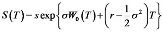
From (3), (4), (5), and (10), we have the time T stock price

(46)

and the time T state price density

(47)

To apply the -hedging approach, one needs an expression for, which according to (45), is given by

(48)

From the formulae (3) and (10), can be written in terms of by

where

.

Let us put. The expression (48) can be rewritten as

(49)

Note that is independent of and is -measurable. By the basic properties of the Brownian motion, we can rewrite (49) as

(50)

where is the normal density function with mean

and variance. To proceed with the -hedging approach, one has to assume that (50) is a function of. However, in general, (50) may not have a closed-form expression. Furthermore, notice that the integrand in (50) is not even once differentiable. Therefore, the assumption that (50) is seems hard to verify. Nevertheless, for comparison purpose, we ignore this technical difficulty for now and pursue the -hedging formula. Assuming that the differentiation can be carried out under the integral sign, we obtain

(51)

(52)

where the set. Recall the relationship. After further simplifications, we have

(53)

We now derive the partial hedging portfolio using the Malliavin calculus approach. The following properties, which are proved in the Appendix, hold.

Corollary 5.1 belongs to and

where the set.

From Corollary 5.1 and Theorem 4.1, the replicating portfolio is given by

(54)

which coincides with the hedging formula in (53). Notice that the Malliavin calculus approach not only avoids the technical difficulty encountered by the -hedging approach, but also uses much less derivation work.

Example 5.2 Now let us consider deriving the partial hedging portfolio for a standard lookback put option with terminal payoff where

. The optimal terminal wealth is given by

(55)

To pursue the -hedging approach, one needs an expression for the optimal wealth process

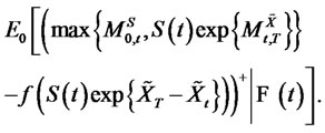
(56)

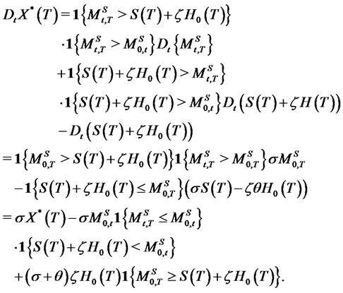
In the Appendix, we show that (56) can be rewritten as

(57)

where and is given in (68). First of all, it is very hard, if not impossible to obtain a closed-form expression for (57). Furthermore, the integrand in (57) is not differentiable with respect to. Therefore, verification of the differentiability condition is not easy. Even if we ignore this technical difficulty, formal differentiation (disregarding the points where it is non-differentiable) would be possible but gets algebraically very messy in addition to being non-rigorous. For these reasons we abandon the delta-hedging approach and pursue the Malliavin calculus approach instead.

Corollary 5.2 Let the optimal terminal wealth be defined by. Then and

Proof. See Appendix.

It then follows from Theorem 4.1 and Corollary 5.2 that the replicating portfolio is given by

(58)

Define the Radon-Nikodym derivative

such that is a probability measure absolutely continuous with respect to. By the Girsanov theorem, the process is a Brownian motion under the probability measure. Moreover, from Lemma 8.6.2 in [14], it follows that for every stochastic variable such that,

(59)

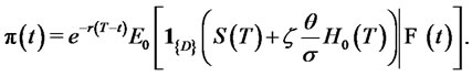
Now the last conditional expectation on the right hand side of Equation (58) can be written as

(60)

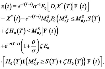
Formulae (58) and (60) yield the optimal partial hedging strategy

(61)

6. Conclusion

We solved the stochastic control problem of minimizing the expected shortfall risk (quantified by a general convex risk measure) under the constraint that the initial capital is insufficient for a perfect hedge. We showed by examples that the Malliavin calculus approach is useful for finding the replicating portfolios in the partial hedging environment. Further research consists of investigating other target contingent claims and extending the results to incomplete markets.

REFERENCES

Appendix

Proof of Lemma 3.1.

Let By the market completeness there exists a such that If then satisfies the statement of the lemma. Suppose that. By Dudley’s theorem ([16] or [17], Theorem 3.4.20) there exists a process satisfying

and

Let

and. It follows that

(62)

and for every

(63)

Let. Relations (9), (62), and (63) imply that

(64)

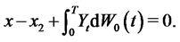
Finally we define. We have since

By (64)

Proof of Corollary 5.1. From Corollary 1 in [7], we know that

belongs to the Banach space and

. To show

and, we approximate by a sequence in and use Definition 4.1 together with the closability of the Malliavin derivative. Notice also that both and are absolutely continuous. Then must, as the difference of absolutely continuous functions, be absolutely continuous. Since is a piecewise Lipschitz function for all x, it follows from Proposition 4.1 that with

Derivation of Expression (57). We are going to derive an expression for the conditional expectation

(65)

Expression (57) can then be obtained by multiplying the above conditional expectation by. Equations (3) and (10) imply the relation

Recall the definition for the function

.

Then (65) can be written as

(66)

Define the notations and. Then can be written as. Recall the notation

. In conjunction with the expression, for, it follows that. Therefore (66) can be written as

(67)

We note that and are independent of, whereas and are -measurable. By the well-known properties of the Brownian motion, the joint distribution of coincides with that of. It is known (see [15], Corollary B.3.1, p. 469) that

(68)

for such that and. We can now write (67) as

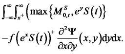(69)

The expression (57) is obtained by multiplying (69) by.

Proof of Corollary 5.2. Write as

where. From Corollary 1 in [7] and Corollary 5.1 above, , , and all belong to. Now as is a Lipschitz function for all x, y, and z, we have by Proposition 4.1 that,and as the joint law of

is absolutely continuous with respect to the Lebesgue measure on we get that

REFERENCES

- J. Cvitanic and I. Karatzas, “On Dynamic Measures of Risk,” Finance and Stochastics, Vol. 3, No. 4, 1999, pp. 451-482. doi:10.1007/s007800050071
- J. Cvitanic, “Minimizing Expected Loss of Hedging in Incomplete and Constrained Markets,” SIAM Journal on Control and Optimization, Vol. 38, No. 4, 2000, pp. 1050-1066. doi:10.1137/S036301299834185X
- H. Föllmer and P. Leukert, “Efficient Hedging: Cost Versus Shortfall Risk,” Finance and Stochastics, Vol. 4, No. 2, 2000, pp. 117-146. doi:10.1007/s007800050008
- H.-P. Bermin, “Hedging Options: The Malliavin Calculus Approach Versus the
-Hedging Approach,” Mathematical Finance, Vol. 13, No. 1, 2003, pp. 73-84. doi:10.1111/1467-9965.t01-1-00006
- D. Ocone and I. Karatzas, “A Generalized Clark Representation Formula with Applications to Optimal Portfolios,” Stochastics and Stochastic Reports, Vol. 34, No. 3- 4, 1991, pp. 187-220.
- P. Lakner, “Optimal Trading Strategy for an Investor: The Case of Partial Information,” Stochastic Processes and Their Applications, Vol. 76, No. 1, 1998, pp. 77-97. doi:10.1016/S0304-4149(98)00032-5
- H.-P. Bermin, “Hedging Lookback and Partial Lookback Options Using Malliavin Calculus,” Applied Mathematical Finance, Vol. 7, No. 2, 2000, pp. 75-100. doi:10.1080/13504860010014052
- H.-P. Bermin, “A General Approach to Hedging Options: Applications to Barrier and Partial Barrier Options,” Mathematical Finance, Vol. 12, No. 3, 2002, pp. 199-218. doi:10.1111/1467-9965.02007
- P. Lakner and L. M. Nygren, “Portfolio Optimization with Downside Constraints,” Mathematical Finance, Vol. 16, No. 2, 2006, pp. 283-299. doi:10.1111/j.1467-9965.2006.00272.x
- F. Black and M. Scholes, “The Pricing of Options on Corporate Liabilities,” Journal of Political Economy, Vol. 81, No. 3, 1973, pp. 637-659. doi:10.1086/260062
- V. Bawa, “Optimal Rules for Ordering Uncertain Prospects,” Journal of Financial Economics, Vol. 2, No. 1, 1975, pp. 95-121. doi:10.1016/0304-405X(75)90025-2
- I. Karatzas and S. E. Steven, “Methods of Mathematical Finance,” Springer-Verlag, New York, 1998.
- D. Nualart, “The Malliavin Calculus and Related Topics,” Springer-Verlag, Berlin Heidelberg, New York, 1995.
- B. K. Oksendal, “Stochastic Differential Equations: An Introduction with Applications,” 5th Edition, SpringerVerlag, Berlin Heidelberg, New York, 1998.
- M. Musiela and M. Rutkowski, “Martingale Methods in Financial Modelling,” Springer-Verlag, Berlin Heidelberg, 1997.
- R. M. Dudley, “Wiener Functionals as Itô Integrals,” Annals of Probability, Vol. 5, No. 1, 1977, pp. 140-141. doi:10.1214/aop/1176995898
- I. Karatzas and S. E. Shreve, “Brownian Motion and Stochastic Calculus,” Springer-Verlag, New York, 1991. doi:10.1007/978-1-4612-0949-2