Consistency of the Model Order Change-Point Estimator for GARCH Models

Irene W. Irungu^1*, Peter N. Mwita², Antony G. Waititu³

¹Pan-African University Institute of Basic Sciences, Technology and Innovatio, Nairobi, Kenya.
²Machakos University, Machakos, Kenya.
³Jomo Kenyatta University of Agriculture and Technology, Nairobi, Kenya.

DOI: 10.4236/jmf.2018.82018                

Abstract

GARCH models have been commonly used to capture volatility dynamics in financial time series. A key assumption utilized is that the series is stationary as this allows for model identifiability. This however violates the volatility clustering property exhibited by financial returns series. Existing methods attribute this phenomenon to parameter change. However, the assumption of fixed model order is too restrictive for long time series. This paper proposes a change-point estimator based on Manhattan distance. The estimator is applicable to GARCH model order change-point detection. Procedures are based on the sample autocorrelation function of squared series. The asymptotic consistency of the estimator is proven theoretically.

Keywords

Autocorrelation Function, Change-Point, Consistency, GARCH, Manhattan Distance, Model Order

1. Introduction

Modelling volatility of financial asset returns is particularly an important area in Finance. This is because volatility is considered to be a measure of risk when pricing financial instruments. The series particularly is characterized by the property of volatility clustering and thus can be considered to display a stationary behavior for some time then suddenly the variability changes, it stays constant for some time at this new value until another change occurs. This therefore suggests that the financial returns series is non-stationary and can be looked at as a union of several stationary series. GARCH models have been commonly used to capture volatility dynamics in financial time series particularly in modelling of stock market volatility as seen in [1] [2] [3] and derivative market volatility as utilized by [4] [5] and [6] .

Given the changing pace of the underlying economic mechanism and technological progress, modeling economic processes over a long time horizon, it is possible that structural changes may occur. This can cause the time series to deviate from stationarity and result to volatility clustering. The detection of these structural change points is therefore vital to various players in a given economy to ensure timeliness of decisions. A fundamental problem in financial trading is the correct and timely identification of turning points in stock value series. This detection enables one to make profitable investment decisions, such as buying-at-low and selling-at-high, hence traders require early identification of local troughs and peaks of stock values. In macroeconomics, knowing the beginning of a recession leads to an increase of government expenditure or an expansion of money supply.

A key assumption of the GARCH models used is that the process is stationary as this allows for model identifiability. However, this violates the volatility clustering property exhibited by the financial returns series. This phenomenon is manifested by the fact that the absolute value of returns or their squares display a positive, significant and slowly decaying autocorrelation function despite the fact that the returns are uncorrelated. This indicates that modeling financial returns series over long time horizons deviates from the stationarity assumption suggesting the existence of a change-point in the series. A modification of the GARCH model, specifically the IGARCH model, has been proposed to model the persistent changes in volatility as the stationarity assumption is relaxed. However the IGARCH model is prone to some shortcomings. [7] showed that the behavior of an IGARCH process depends on the intercept, such that, if the intercept is positive then the unconditional variance of the process grows linearly with time. In practice this means that the amplitude of the clusters of volatility to be parametrized by the model on the average increases over time. The rate of increase needs not, however, be particularly rapid. If the intercept is zero in the IGARCH model, the realizations from the process collapse to zero almost surely. However, a potentially disturbing fact is that the model assumes that the unconditional variance of the process to be modeled does not exist in that the variance may be infinite [8] and [9] .

It is argued that in applications, the assumption of parameter constancy in GARCH models may not be appropriate especially when the series to be modeled are long [10] . To overcome this problem of modeling financial time series in the presence of structural changes, the duo suggests that one option is to assume that the parameters change at specific points of time, divide the series into sub-series according to the location of the change-points and fit separate GARCH models to the sub-series. This brings about the challenge of determining the number of change-points and their location because they are normally not known in advance. This proposition has been adopted by various researchers who have utilized different methodologies to be able to locate the change-points attributed to change in parameter specification. The use of squared model residuals and likelihood ratio to detect parameter changes is proposed by [11] while [12] proposes the use of Markov-switching GARCH models estimated through Markov Chain Monte Carlo simulation methods. Modeling of equity volatilities as a combination of macroeconomic effects and time series dynamics by combining exponential splines and GARCH models is utilized by [13] . An alternative approach is to use smooth transition GARCH model. This can be achieved by defining a transition function where the coefficients are expressed as a function of time as in [9] or by employing non-linear functions that are lagged for the squared observations [14] and [15] or lagging the conditional variance [16] . CUSUM tests have also been proposed as suitable methods of identifying change-points by establishing breaks in moments of the time series. The use of the unconditional variance is proposed by [17] while [18] [19] use the mean. However, these methods are mainly based on the assumption that change-points occur solely due to change in parameter specification. The approach presented here seeks to identify change-points attributed to change in model order specification.

This paper is organized as follows. Section 2 gives an overview of GARCH model specification with corresponding assumptions utilized in the proof of the main result. Section 3 presents the proposed change-point estimator for change attributed to in the model orders p and q in GARCH models. The estimator is based on the Manhattan distance of sample autocorrelations of a squared returns series. Section 4 provides proof of the consistency of the proposed change-point estimator.

2. GARCH Model

Assume that the data $X_t$ , for $t\in \mathbb{Z}$ , are independent and sampled at equi-spaced points. The series ${\left(X_t\right)}_{t\in \mathbb{Z}}$ describe a financial returns time series modeled using $\text{GARCH}\left(p,q\right)$ model specified as:

$\begin{array}{l}{X}_t={\sigma }_t{ϵ}_t\text{for}t\in \mathbb{Z}\\ {\sigma }_t^2={\alpha }_0+\underset{i=1}{\overset{p}{{\displaystyle \sum }}}{\alpha }_i{X}_{t-i}^2+\underset{j=1}{\overset{q}{{\displaystyle \sum }}}{\beta }_j{\sigma }_{t-j}^2\end{array}$ (1)

The sequence of innovations ${\left({ϵ}_t\right)}_{t\in \mathbb{Z}}$ is an independent and identically distributed (iid) sequence with mean zero and unit variance. ${\left({\sigma }_t\right)}_{t\in \mathbb{Z}}$ is the volatility sequence of the GARCH model. Assume that ${\alpha }_p{\beta }_q\ne 0$ and that all coefficients ${\alpha }_i$ and ${\beta }_j$ are non-negative to avoid ambiguity with regards to orders $\left(p,q\right)$ . Since we are not interested in the trivial solution $X_t\equiv 0$ to (1), further assume that ${\alpha }_0>0$ .

Let $p=q$ and $c_{i,t-i}={\beta }_i+{\alpha }_i{ϵ}_{t-i}^2$ for $i=1,2,\cdots ,p$ , where $\left\{c_{i,t}\right\}$ is a sequence of independent and identically distributed random variables such that $c_{i,t}$ is independent of ${\sigma }_t$ . This allows us to rewrite (1) as

$\begin{array}{l}{X}_t={\sigma }_t{ϵ}_t\text{for}t\in \mathbb{Z}\\ {\sigma }_t^2={\alpha }_0+\underset{i=1}{\overset{p}{{\displaystyle \sum }}}{\alpha }_i{X}_{t-i}^2+\underset{j=1}{\overset{p}{{\displaystyle \sum }}}{\beta }_j{\sigma }_{t-j}^2\\ ={\alpha }_0+\underset{i=1}{\overset{p}{{\displaystyle \sum }}}\left({\beta }_i+{\alpha }_i{ϵ}_{t-i}^2\right){\sigma }_{t-i}^2\\ ={\alpha }_0+\underset{i=1}{\overset{p}{{\displaystyle \sum }}}{c}_{i,t-i}{\sigma }_{t-i}^2\end{array}$ (2)

Model (2) is utilized in the proof of consistency of the proposed change-point estimator.

The GARCH (p,q) model (1) can also be represented as an ARMA(max(p,q),q) as showed by [20] as

$X_t^2-\underset{i=1}{\overset{p}{{\displaystyle \sum }}}{\alpha }_i{X}_{t-i}^2-\underset{j=1}{\overset{q}{{\displaystyle \sum }}}{\beta }_j{X}_{t-j}^2={\alpha }_0+u_t-\underset{j=1}{\overset{q}{{\displaystyle \sum }}}{\beta }_j{u}_{t-j}\text{for}t\in \mathbb{Z}$ (3)

where $u_t=X_t^2-{\sigma }_t^2$ and  ${\left(u_t\right)}_{t\in \mathbb{Z}}$ is white noise.

This representation of the GARCH model follows the standard ARMA form for the squared series, therefore, conventional methods used to identify ARMA processes may be used to determine the presence of GARCH. Of keen interest is the use of the sample autocorrelation function (SACF) and partial autocorrelation functions (PACF). Specifically, the orders p and q are drawn from the autocorrelation function and partial autocorrelation function respectively. Empirically, these orders are chosen such that the SACF cuts off after lag p and the PACF decline exponentially to zero after lag q for which they are significant. In light of this it can be asserted that the SACF and PACF can be used to distinguish GARCH model with different model orders specifications.

The following assumptions are necessary to prove the subsequent theoretical results.

Assumption 1 (Independence)

i) ${ϵ}_t$ ’s are independent and identically distributed

ii) $X_t$ ’s are independent of the ${ϵ}_t$ ’s for $1\le t\le n$

Assumption 1 will ensure parameters in model (1) are estimated using Quasi-Maximum Likelihood Estimation method.

Assumption 2 (Strictly Stationary)

According to [21] the existence of a unique strictly stationary solution to (1) is the negativity of the top Lyapunov exponent. This however cannot be calculated explicitly but a sufficient condition for this is given by

$\underset{i=1}{\overset{p}{{\displaystyle \sum }}}{\alpha }_i+\underset{j=1}{\overset{q}{{\displaystyle \sum }}}{\beta }_j<1$ (4)

Assumption 3 (Ergodic Process)

According to [22] standard ergodic theory yields that $\left(X_t\right)$ is an ergodic process. Thus its properties can be deduced from a single sufficiently large random sample of the sample.

3. Change-Point Estimator

Assume that the data ${\left\{X_t\right\}}_{t=1}^n$ describes a financial returns time series modeled using $\text{GARCH}\left(p,q\right)$ process. A single change-point testing problem is first considered where it is assumed that a change-point can happen only at time k where $1<k<n-1$ . The hypotheses to be investigated are assumed to follow the following definition:

$\begin{array}{l}{H}_0:X_t\sim \text{GARCH}\left(1,1\right)\text{for}t=1,\cdots ,n\\ \text{against}\\ H_1:X_t\sim \{\begin{array}{l}\text{GARCH}\left(1,1\right)\text{for}t=1,\cdots ,k\\ \text{GARCH}\left(p,q\right)\text{for}t=k+1,\cdots ,n\end{array}\text{where}p,q\in \mathbb{N}\backslash \left\{0\right\}\end{array}$ (5)

Let $I=\mathbb{N}$ be a finite index sequence and ${\left(X_t\right)}_{t\in \mathbb{N}}$ satisfy Assumptions 1 and 2. Let $X=\left(X_1,X_2,\cdots ,X_k\right)$ be a k dimensional vector and $Y=\left(X_{k+1},X_{k+2},\cdots ,X_n\right)$ be a $\left(n-k\right)$ dimensional vector. The autocovariance and autocorrelation functions can be expressed in terms of the inner product as

$acovar\langle X,Y\rangle =\langle X-E\left(X\right),Y-E\left(Y\right)\rangle$ (6)

$acorr\langle X,Y\rangle =\langle \frac{X-E\left(X\right)}{sd(X)},\frac{Y-E\left(Y\right)}{sd\left(Y\right)}\rangle$ (7)

where $sd\left(X\right)$ and $sd\left(Y\right)$ represents the standard deviation of X and Y respectively which represents an $L_2$ distance from the mean.

By the Assumption 3 that the series ${\left(X_t\right)}_{t\in \mathbb{N}}$ is ergodic, then it is implied that the sample moments converge in probability to the population moments. It therefore follows that the sample autocovariance and autocorrelation converge in probability to the population autocovariance and autocorrelation respectively.

Theorem 1. (Holder’s Inequality)

Let I be a finite or countable index set. Given $1\le p\le \infty$ , if $X={\left(X_k\right)}_{k\in I}\in L_p\left(I\right)$ and $Y={\left(Y_k\right)}_{k\in I}\in L_{p^{\prime }}\left(I\right)$ , where $\frac{1}{p}+\frac{1}{p^{\prime }}=1$ then $XY={\left(X_k{Y}_k\right)}_{k\in I}\in L_1\left(I\right)$ and

${\Vert XY\Vert }_1\le {\Vert {\left(X_k\right)}_{k\in I}\Vert }_p{\Vert {\left(Y_k\right)}_{k\in I}\Vert }_{p^{\prime }}={\left(\underset{k\in I}{{\displaystyle \sum }}{\left|X_k\right|}^p\right)}^{\frac{1}{p}}{\left(\underset{k\in I}{{\displaystyle \sum }}{\left|Y_k\right|}^{p^{\prime }}\right)}^{\frac{1}{p^{\prime }}}<\infty$ (8)

Let $p=p^{\prime }=2$ in the Holders Inequality Theorem 1 we obtain

$E\left(\left|X\right|\left|Y\right|\right)\le \sqrt{E\left(X^2\right)}\sqrt{E\left(Y^2\right)}$ (9)

Thus, applying the result in (9) to (6) and (7) yields

$\left|acovar\left(X,Y\right)\right|\le sd\left(X\right)sd\left(Y\right)\in L_1\text{space}$ (10)

$\left|acorr\left(X,Y\right)\right|\le 1\in L_1\text{space}$ (11)

Following (11) define sequences of autocorrelation functions ${\rho }_{i+1,j}$ where for fixed $i=0$ , $1\le j\le n-1$ and for fixed $j=n$ , $1\le i\le n-1$ to be such that we have two subsequences ${\rho }_{1j}=\left({\rho }_{1,1},{\rho }_{1,2},\cdots ,{\rho }_{1,k},\cdots {\rho }_{1,n-1}\right)$ and

${\rho }_{in}=\left({\rho }_{2,n},{\rho }_{3,n},\cdots ,{\rho }_{k+1,n},\cdots ,{\rho }_{nn}\right)$ where ${\rho }_{1,k}$ and ${\rho }_{k+1,n}$ denote the autocorrelation of the sequence ${\left\{X_t^2\right\}}_{t=1}^k$ and ${\left\{X_t^2\right\}}_{t=k+1}^n$ for $1\le k\le n$ .

An estimator is proposed drawn from a process $D_n^k$ quantifying the deviation between ${\rho }_{1,k}$ and ${\rho }_{k+1,n}$ using a divergence measure motivated by the weighted $L_p$ distance, with k denoting the change-point. For $p>0$ define

$\begin{array}{l}{L}_p\left({\rho }_{1,k}-{\rho }_{k+1,n}\right)={\left(\underset{k=1}{\overset{n}{{\displaystyle \sum }}}{w}_k{\left|{\varphi }_k-{\varphi }_{k+1}\right|}^p\right)}^{\frac{1}{p}}\\ \text{where}{\varphi }_k=\frac{{{\displaystyle \sum }}_{t=1}^{k-h}{X}_t^2{X}_{t+h}^2}{{{\displaystyle \sum }}_{t=1}^k{X}_t^4}\text{for}0<k<n,0<h<n\end{array}$ (12)

Specifically, assume the case when $p=1$ in (12) resulting into a weighted Manhattan distance and by linearity and absolute value of inequalities of the expectation operator results into

$\begin{array}{c}{L}_1\left({\rho }_{1,k}-{\rho }_{k+1,n}\right)=\left(\underset{k=1}{\overset{n}{{\displaystyle \sum }}}{w}_k\left|{\varphi }_k-{\varphi }_{k+1}\right|\right)\\ =E\left(w_k\left|{\varphi }_k-{\varphi }_{k+1}\right|\right)\\ \ge w_k\left|E\left({\varphi }_k\right)-E\left({\varphi }_{k+1}\right)\right|\end{array}$ (13)

To facilitate the construction of the proposed estimator the lower bound of the divergence measure (13) is assumed. Further assume that the autocorrelation function is calculated at lag $h:0<h<n$ . The proposed change-point estimator is thus developed from the process generated by this measure as follows:

$w_k\left|E\left({\varphi }_k\right)-E\left({\varphi }_{k+1}\right)\right|=w_k\left|\frac{1}{k}\underset{i=1}{\overset{k}{{\displaystyle \sum }}}{\varphi }_i-\frac{1}{n-k}\underset{i=k+1}{\overset{n}{{\displaystyle \sum }}}{\varphi }_i\right|$ (14)

From (14) it can be seen that the proposed test is a weighted difference between the sample autocorrelation functions ${\rho }_{1,k}$ and ${\rho }_{k+1,n}$ with $\begin{array}{c}{w}_k\end{array}$ denoting the weight.

Assumption 4. (Weight)

The weight $\begin{array}{c}{w}_k\end{array}$ is a measurable function that depends on the sample size n and change-point . It is arbitrarily chosen such that it satisfies the condition that

$\begin{array}{l}\underset{i=1}{\overset{k}{{\displaystyle \sum }}}{\varphi }_i=\frac{k}{n}\underset{i=1}{\overset{n}{{\displaystyle \sum }}}{\varphi }_i\\ \Rightarrow \frac{1}{n}\left(\underset{i=1}{\overset{k}{{\displaystyle \sum }}}{\varphi }_i-\frac{k}{n}\underset{i=1}{\overset{n}{{\displaystyle \sum }}}{\varphi }_i\right)=0\end{array}$ (15)

Equating (14) and (15) determines the weight $w_k$ as follows:

$\begin{array}{l}{w}_k\left(\frac{1}{k}\underset{i=1}{\overset{k}{{\displaystyle \sum }}}{\varphi }_i-\frac{1}{n-k}\underset{i=k+1}{\overset{n}{{\displaystyle \sum }}}{\varphi }_i\right)=\frac{1}{n}\left(\underset{i=1}{\overset{k}{{\displaystyle \sum }}}{\varphi }_i-\frac{k}{n}\underset{i=1}{\overset{n}{{\displaystyle \sum }}}{\varphi }_i\right)\\ =\frac{1}{n}\left(\left[1-\frac{k}{n}\right]\underset{i=1}{\overset{k}{{\displaystyle \sum }}}{\varphi }_i-\frac{k}{n}\underset{i=k+1}{\overset{n}{{\displaystyle \sum }}}{\varphi }_i\right)\left(\frac{k}{k}\right)\left(\frac{n-k}{n-k}\right)\end{array}$

$\begin{array}{l}=\frac{k}{n}\left(1-\frac{k}{n}\right)\left(\frac{1}{k}\underset{i=1}{\overset{k}{{\displaystyle \sum }}}{\varphi }_i-\frac{1}{n-k}\underset{i=k+1}{\overset{n}{{\displaystyle \sum }}}{\varphi }_i\right)\\ \Rightarrow w_k=\frac{k}{n}\left(1-\frac{k}{n}\right)\end{array}$ (16)

The resultant process is obtained from (14) and (16) and defined as

$D_n^k=\frac{k}{n}\left(1-\frac{k}{n}\right)\left|\frac{1}{k}\underset{i=1}{\overset{k}{{\displaystyle \sum }}}{\varphi }_i-\frac{1}{n-k}\underset{i=k+1}{\overset{n}{{\displaystyle \sum }}}{\varphi }_i\right|$ (17)

The change-point estimator $\hat{k}$ of a change point $k^{*}$ is the point at which there is maximal sample evidence for a break in the sample autocorrelation function of the squared returns process. It is therefore estimated as the least value of k that maximizes the value of $D_n^k$ where $1<k<n$ is chosen as:

$\hat{k}=\min \left\{k:D_n^k=\underset{1<k<n}{\max }\left|D_n^k\right|\right\}$ (18)

4. Simulation Study

The performance of the proposed estimator is examined by considering the effects of the change in sample size. Assume that $\left\{X_t\right\}$ is a stationary $\text{GARCH}\left(p,q\right)$ process where $p,q\in \mathbb{N}\backslash \left\{0\right\}$ . The single change-point estimation

problem is considered where the change-point k is fixed at $\frac{n}{2}$ for $n=500$ ,

$n=1000$ and $n=2000$ . Figures 1-3 display the plots for the location of the change-point estimator as estimated by the proposed estimator (18) for various sample sizes. The hypothesis considered here is when change occurs in model order q, described as;

$\begin{array}{l}{H}_0:X_t\sim \text{GARCH}\left(1,1\right)\text{for}t=1,\cdots ,n\\ \text{against}\\ H_1:X_t\sim \text{GARCH}\left(1,1\right)\text{for}t=1,\cdots ,k\\ X_t\sim \text{GARCH}\left(1,2\right)\text{for}t=k+1,\cdots ,n\end{array}$ (19)

The following table gives the parameter estimates used in the simulation.

The change-point estimators obtained are $k=264$ , $k=587$ and $k=1052$ for sample sizes 500, 1000 and 2000 respectively as displayed in Figures 1-3. The performance of the estimators is evaluated using the Adjusted Rand Index (ARI) which compares the segmentation created by the change-point estimator and the true segmentation. The Adjusted Rand Index lies between 0 and 1. When the two partitions agree perfectly, the ARI is 1. The results of the ARI are provided in Table 1 for changes in order q.

The results for the change in order q in Table 1 show that as the sample size increases, the similarity index given by ARI generally increases.

5. Consistency of the Change-Point Estimator

Consider a sample $X_1^2,X_2^2,\cdots ,X_n^2$ satisfying (2) and (5) and the change-point estimator $\hat{k}$ given by (18). If the sequences $\left\{X_{1,k}^2\right\}$ and $\left\{X_{2,k}^2\right\}$ satisfy

Figure 1. Single Change-Point for Stationary Series GARCH $X_t$ for $n=500.$

Figure 2. Single Change-Point for Stationary Series GARCH $X_t$ for $n=1000.$

Figure 3. Single Change-Point for Stationary Series GARCH $X_t$ for $n=2000.$

Table 1. Adjusted rand index given changes in order q.

$\begin{array}{l}\delta =\frac{{\nu }_2{\gamma }_{11}^{h-1}\left[{\bar{\gamma }}_{11}\left(1-{\gamma }_{11}^2\right)-{\nu }_2{\gamma }_{11}\left(1-{\gamma }_{12}\right)\right]}{{\nu }_4\left(1-{\gamma }_{11}^2\right)-{\nu }_2^2\left(1-{\gamma }_{12}\right)}\\ -\frac{{\nu }_2{\gamma }_{S_1}\left(1-{\gamma }_1\right)M_2\left(h\right)-{\nu }_2^2{\gamma }_{S_2}\left[1-\left(1-{\gamma }_1\right)M_1\left(h\right)\right]}{{\nu }_4{\gamma }_{S_1}\left(1-{\gamma }_1\right)-{\nu }_2^2{\gamma }_{S_2}}\ne 0\end{array}$ (20)

then for $\hat{\tau }=\frac{\hat{k}}{n}$ ,

$P\left\{\left|\hat{\tau }-{\tau }^{*}\right|>\epsilon \right\}\le \frac{C}{{\epsilon }^2{\delta }^2{n}^{\frac{1}{2}}}$ (21)

where C is a positive constant.

Proof Suppose that $\left\{X_{1,k}^2,k\in \mathbb{Z}\right\}$ and $\left\{X_{2,k}^2,k\in \mathbb{Z}\right\}$ are two $\text{GARCH}\left(p,q\right)$ sequences as defined in model (2). Further suppose that a sample $X_1^2,X_2^2,\cdots ,X_n^2$ from the model is observed, such that

$X_k^2=\{\begin{array}{l}{X}_{1,k}^2\text{if}1\le k\le k^{*}\\ X_{2,k}^2\text{if}{k}^{*}<k\le n\end{array}$ (22)

where $k^{*}$ is the unknown change point. More specifically assume that the two sequences have different model order specification such that

$X_k^2=\{\begin{array}{l}\text{GARCH}\left(p_1,q_1\right)\text{if}1\le k\le k^{*}\\ \text{GARCH}\left(p_2,q_2\right)\text{if}{k}^{*}<k\le n\end{array}$ (23)

where $p_1\ne p_2$ and $q_1\ne q_2$ but $p_1=q_1=1$ and $p_2=q_2$ . Let $k^{*}={\tau }^{*}n$ and assume that $0<\tau <1$ , then in the presence of the change-point, the sequence $\left\{X_k^2\right\}$ is no longer stationary.

The foundation of this proof is based on the second and fourth moments of $\left\{X_t\right\}$ which will first be derived. Assume that the GARCH(p,p) model (2) has a finite fourth moment and let $E\left({ϵ}_t^j\right)={\nu }_j,j=2,4$ . The assumption that the second moment of $\left\{X_t\right\}$ exist it implies that $E\left(c_{i,t-i}\right)={\beta }_i+{\alpha }_i{\nu }_2<1$ . Let ${\gamma }_{i1}=E\left(c_{i,t-i}\right)$ , ${\gamma }_{i2}=E\left(c_{i,t-i}^2\right)$ and ${\gamma }_i={\displaystyle {\sum }_{i=1}^p{\gamma }_{ij}}$ for $i=1,2,\cdots ,p$ and $j=1,2$ . The second and fourth moments of $\left\{X_t\right\}$ is established by determining $E\left({\sigma }_t^2\right)$ and $E\left({\sigma }_t^4\right)$ as follows:

$E\left({\sigma }_t^2\right)=E\left({\alpha }_0+\underset{i=1}{\overset{p}{{\displaystyle \sum }}}{c}_{i,t-i}{\sigma }_{t-i}^2\right)=\frac{{\alpha }_0}{1-{\gamma }_1}$ (24)

Equation (24) shows is that $E\left({\sigma }_t^2\right)<\infty$ exists for ${\gamma }_1<1$ .

$\begin{array}{c}E\left({\sigma }_t^4\right)=E\left({\alpha }_0^2+2{\alpha }_0\underset{i=1}{\overset{p}{{\displaystyle \sum }}}{c}_{i,t-i}{\sigma }_{t-i}^2+\underset{i=1}{\overset{p}{{\displaystyle \sum }}}{c}_{i,t-i}^2{\sigma }_{t-i}^4+2\underset{l<m}{\overset{p}{{\displaystyle \sum }}}{c}_{l,t-l}{c}_{m,t-m}{\sigma }_{t-l}^2{\sigma }_{t-m}^2\right)\\ ={\alpha }_0^2+2{\alpha }_0{\gamma }_{1}E\left({\sigma }_t^2\right)+{\gamma }_{2}E\left({\sigma }_t^4\right)+2\underset{l<m}{\overset{p}{{\displaystyle \sum }}}E\left(c_{l,t-l}{c}_{m,t-m}{\sigma }_{t-l}^2{\sigma }_{t-m}^2\right)\end{array}$ (25)

To establish $E\left({\sigma }_t^4\right)$ the $E\left(c_{l,t-l}{c}_{m,t-m}{\sigma }_{t-l}^2{\sigma }_{t-m}^2\right)$ is determined using the following Theorems as proved by [23] .

Theorem 2. Assume that $\lambda \left(\Gamma \right)<1$ . Under this condition,

$E\left(c_{l,t-l}{c}_{m,t-m}{\sigma }_{t-l}^2{\sigma }_{t-m}^2\right)={\alpha }_0{\gamma }_{l1}{\gamma }_{m1}{M}_1\left(l,m\right)E\left({\sigma }_t^2\right)+{\gamma }_{l1}{M}_2\left(l,m\right)E\left({\sigma }_t^4\right)$ (26)

where for $m-l>1$

$M_1\left(l,m\right)=1+{{\gamma }^{\prime }}_{P\backslash \left\{m-l\right\}}\left[\underset{i=1}{\overset{m-l-1}{{\displaystyle \sum }}}\left(\underset{j=1}{\overset{i}{{\displaystyle \prod }}}{\Gamma }_j\right)e_1+\underset{i=1}{\overset{m-l}{{\displaystyle \prod }}}{\Gamma }_i\left(j_{p-1}+{\Gamma }_{m-l+1}{\left(I_{p^{*}}-\Gamma \right)}^{-1}{e}_{p-1}\right)\right]$

$j_{p-1}={\left(1,1,\cdots ,1\right)}^{\prime }$ is a $\left(p-1\right)\times 1$ vector

$e_{p-1}={\left(1,\cdots ,1,0,\cdots ,0\right)}^{\prime }$ is a vector with the first elements equal to 1

is a matrix of order with a matrix of order and Γ a matrix of order

is maximum absolute eigenvalue of the matrix Γ

In particular

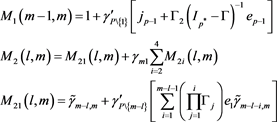
Proof. For proof of Theorem 2 see Appendix 5 of [23] .

Substituting (24) and (26) in (25) yields

(27)

(28)

From (28) it can be deduced that for and.

Now the fourth moment of is evaluated as

(29)

Equation (29) implies that fourth moment of exist if and.

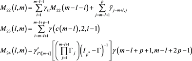
The mixed moment has the form

(30)

where for,

Proof. For proof of Theorem 2 see Appendix 9 of [23] .

The expected value of the sample autocorrelation function, , is first evaluated using (29) and (30).

(31)

Further assuming that (22) and (23) are satisfied, evaluate (31) for as follows:

(32)

(33)

For GARCH(1,1) model,. Substituting (37) and (33) in (31) results to

(34)

Equation (34) shows that, in the presence of a change-point, the expected value of the sample autocorrelation function before and after the true change-point is not equal. We consider a special case of change from GARCH(1,1) to GARCH(2,2) where we evaluate (31) for as follows:

(35)

(36)

Applying Theorem 3 and letting yields

The expected value, , for (23) for model order specification and for lag 1 results to

(37)

From (34) and (37), it can be seen that in the presence of a change-point then

(38)

To proof consistency of the estimator we need to show that as the sample size n increases. Thus the is evaluated noting that it reaches its maximum at the point resulting to

(39)

Thus

(40)

From (39) and (40) it follows that

(41)

We also have that

(42)

Thus from (41) and (50) as well as replacing τ with in (41) we have that

(43)

Consider as given in (17), the estimate is now established as follows

(44)

Theorem 4. Let be any random variables with finite second moments and be any non-negative constants. Then

(45)

Proof. For proof of Theorem 4 see Theorem 4.1 of [24] .

Applying Theorem 4 with, and yields

(46)

implying (47)

Substituting the result in (47) to (53) results to

(48)

As from (48) we can see that, which completes proof. Thus the estimator τ is a consistent estimator of implying that k is a consistent estimator of.

6. Conclusion

In this paper we argue that change in GARCH process can be attributed to model order specification which results into a nonstationary series that depicts real data. Given that possible values for p and q can be arrived through inspection of sample autocorrelation and sample partial autocorrelation os squared series, an estimator for the change-point is derived based on the Manhattan distance. Results based on the similarity index ARI show that the estimator performs better as the size of change increases. We are also able to prove consistency of the estimator theoretically. The proposed estimator can be improved to examine departure from other model order specification other that GARCH(1,1). The next paper will focus on establishing the limiting distribution of the estimator.

Acknowledgements

The authors thank the Pan-African University Institute of Basic Sciences, Technology and Innovation (PAUSTI) for funding this research.

Conflicts of Interest

The authors declare no conflicts of interest.

References

[1]	Liljeblom, E. and Stenius, M. (1997) Macroeconomic Volatility and Stock Market Volatility: Empirical Evidence on Finnish Data. Applied Financial Economics, Taylor and Francis Journals, 7, 419-426.
[2]	Yusof, R.M. and Majid, M.S.A. (2007) Stock Market Volatility Transmission in Malaysia: Islamic versus Conventional Stock Market. Journal of King Abdulaziz University: Islamic Economics, 20, 17-35. https://doi.org/10.4197/islec.20-2.2
[3]	Chinzara, Z. (2010) Macroeconomic Uncertainty and Emerging Market Stock Market Volatility: The Case for South Africa. Working Paper 187, 1-19.
[4]	Manera, M., Nicolini, M. and Vignati, I. (2012) Financial Speculation in Energy and Agriculture Futures Markets: A Multivariate GARCH Approach. International Association for Energy Economics.
[5]	Duan, J.C. (1995) The GARCH Option Pricing Model. Mathematical Finance, 5, 13-32. https://doi.org/10.1111/j.1467-9965.1995.tb00099.x
[6]	Hsieh, K.C. and Ritchkeny, P. (2005) An Empirical Comparison of GARCH Option Pricing Models. Review of Derivative Research, 8, 129-150. https://doi.org/10.1007/s11147-006-9001-3
[7]	Nelson, D.B. (1991) Conditional Heteroskedasticity in Asset Returns: A New Approach. Econometrica, 59, 347-370. https://doi.org/10.2307/2938260
[8]	Terasvirta, T. (2009) An Introduction to Univariate GARCH Models. Springer-Verlag Berlin Heidelberg.
[9]	Polzehl, J. and Spokoiny, V. (2006) Varying Coefficient GARCH versus Local Constant Volatility Modeling. Comparison of the Predictive Power.
[10]	Mikosch, T. and Starica, C. (2004) Nonstationarities in Financial Time Series, the Long-Range Dependence and the IGARCH Effects. Review of Economics and Statistics, 86, 378-390. https://doi.org/10.1162/003465304323023886
[11]	Kokoszka, P. and Teyssi Asre, G. (2002) Change-Point Detection in GARCH Models: Asymptotic and Bootstrap Tests. CORE Discussion Papers 2002065, Universit Ac catholique de Louvain, Center for Operations Research and Econometrics (CORE).
[12]	Luc, B., Arnaud, D. and Jeroen, V.K. (2014) Rombouts. Marginal Likelihood for Markov-Switching and Change-Point GARCH Models. Journal of Econometrics, 178, 508-522. https://doi.org/10.1016/j.jeconom.2013.08.017
[13]	Engle, R.F. and Rangel, J.G. (2008) The Spline-Garch Model for Low-Frequency Volatility and Its Global Macroeconomic Causes. The Review of Financial Studies, 21, 1187-1222. https://doi.org/10.1093/rfs/hhn004
[14]	Hagerud, G. (1997) A New Non-Linear GARCH Model. EFI Economic Research Institute, Stockholm.
[15]	Gonzales-Rivera, G. (1998) Smooth Transition GARCH Models. Studies in Nonlinear Dynamics and Econometrics, 3, 161-178. https://doi.org/10.2202/1558-3708.1041
[16]	Lanne, M. and Saikkonen, P. (2005) Non-Linear GARCH Models for Highly Persistent Volatility. Econometrics Journal, 8, 251-276. https://doi.org/10.1111/j.1368-423X.2005.00163.x
[17]	Inclan, C. and Tiao, G.C. (1994) Use of Cumulative Sums of Squares for Retrospective Detection of Changes of Variance. Journal of the American Statistical Association, 89, 913-923.
[18]	Page, E. (1954) Continuous Inspection Schemes. Biometrika, 14, 100-115. https://doi.org/10.1093/biomet/41.1-2.100
[19]	Kokoszka, P. and Leipus, R. (2000) Change-Point Estimation in ARCH Models. Bernoulli, 6, 513-539. https://doi.org/10.2307/3318673
[20]	Bollerslev, T. (1986) Generalized Autoregressive Conditional Heteroskedasticity. Journal of Econometrics, 31, 307-327. https://doi.org/10.1016/0304-4076(86)90063-1
[21]	Bougerol, P. and Picard, N. (1992) Strict Stationarity of Generalized Autoregressive Processes. Annals of Probability, 20, 1714-1730. https://doi.org/10.1214/aop/1176989526
[22]	Krengel, U. and Brunel, A. (1985) Ergodic Theorems. De Gruyter Studies in Mathematics. De Gruyter.
[23]	He, C. and Terasvirta, T. (1999) Fourth Moment Structure of the GARCH (p,q) Process. Econometric Theory, 15, 824-846. https://doi.org/10.1017/S0266466699156032
[24]	Kokoszka, P. and Leipus, R. (2000) Change-Point Estimation in ARCH Models. Bernoulli, 6, 513-539. https://doi.org/10.2307/3318673