Mathematical Model of HIV-1 Circulating Recombinants Forms in Mali

Mahamadou Alassane¹, Amadou Mahamane¹, Ouaténi Diallo¹, Jérôme Pousin²

¹Département de Mathématiques et d’Informatique, Faculté des Sciences et Techniques, Bamako, Mali.
²Institut National des Sciences Appliquées de Lyon, Lyon, France.

DOI: 10.4236/ojmsi.2015.34015                

Abstract

In this paper, we propose a determinist mathematical model for the co-circulating into two circulating recombinants forms (CRFs) Of HIV-disease in Mali. We divide the sexually active population within three compartments (susceptible, CRF-1 infected and CRF-2 or CRF-12 infected) and study the dynamical behavior of this model. Then, we define a basic reproduction number of the CRF-2 or CRF-12 infected individuals R0 and shown that the CRF-2 or CRF-12 infected-free equilibrium is locally-asymptotically stable if R0 < 1 (thus the CRF-2 or CRF-12 infected becomes extinct in population) and unstable if R0 > 1 (thus the CRF-2 or CRF-12 infected invade in the population). Fur-thermore, we prove that under certain conditions on the parameters of the model the controllability of CRF-2 or CRF-12 infected with regard to the CRF-1 infected. Numerical simulations are given to illustrate the results.

Keywords

Asymptotic Stability, Basic Reproduction Number of the CRF-2 or CRF-12 Infected, Controllability

1. Introduction

AIDS is one of the most deadly diseases caused by a humain immunodeficiency virus (HIV). The virus destroys all the immune system and leaves individuals susceptible to any other infections. The lymphocites (in particular the lymphocites T-CD4) multiplies insade those lymphocites and finally destroy them. When the lymphocytes are reduced to a certain numbers, the immune system stops functioning correctly. Therefore, the individual can catch any kind of disease that might kill him easily because of the failure of the immune system. However, there exist drugs that can slow down the evolution of the virus. HIV is usually transmitted in three different ways: sexual contacts, blood transfusion, and exchange between mother and child during pregnancy, childbirth and breastfeeding.

Humain immunodfiency virus (HIV), the causative agent of AIDS, is classified into types, groups, subtypes and sub-subtypes according to its genetic diversity [1] . Subtypes and sub-subtypes can form additional mosaic forms: circulating recombinant forms (CRFs). To date, at least 49 CRF are recognised in diverse parts of the world (http://www.hiv.lanl.govcontent/sequence/HIV/CRFs/CRFs.html).

We propose in this work a mathematical model which describes the cocirculation of two circulating recombinants forms (CRF-1 and CRF-2) of the HIV-1 in Mali. We suppose that the CRF-1 is not resistant in antiretrovirals and it is in an endemic state in the population, whereas the CRF-2 and CRF-12 which is the recombination of the CRF-1 and CRF-2 resist antiretrovirals.

The population is divided into tree compartments (Figure 1): the susceptible (susceptible individuals for CRF-1 and CRF-2 represented by S), the CRF-1 infected (infected individuals by CRF-1) represented by Y₁ and the CRF-2 or CRF-12 infected (infected individuals by CRF-2 or CRF-12) represented by Y₂.

2. Experimental Motivation and Main Results

Our Model is based on the model proposed in [2] , which takes into account the cocirculating of two strains of influenza. We modified two points: in the first we removed the compartment of immune and after we added the possibility for susceptible one infected by a mutant to go into the compartment of this last one. So we have a model in two circulating recombinants forms. Three compartments are thus defined by the state of the individuals (or) concerning each both circulating recombinant form (CRF-1 and CRF-2). The passage in time of the population size in the different states is governed by a system of differential equation a little more complicated than the standard model. For describing the CRF-1 and CRF-2 transmission, a dynamics between the compartments due to the CRF-1 and CRF-2 has to be specified. Each individual of the population is considered to belong to one of the three compartments: susceptible (denoted by), CRF-1 infected, (denoted by Y₁), CRF-2 or CRF-12 infected (denoted by Y₂).

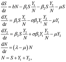
Our model is given by the following system of ODEs:

(1)

where the parameters are defined in Table 1.

Figure 1. Representation of the model.

To analyse the model (7), we introduce the following variables:

Then,. In the new variables, the malaria model (7) becomes

(2)

After normalization of the initial data, we obtain

(3)

and

(4)

The variables of the model (2) are defined in Table 2.

By definition, the variables in Table 2 should satisfy the equation; this is indeed proved in Lemma 2. All the parameters in Table 1 are positive constants. Multiple HIV-1 subtypes and circulating recombinant forms (CRFs) are known to circulate in Africa. In west Africa, the high prevalence of CRF02-AG, and cocirculation of subtype A, CRF01-AE, CRF06-cpx and other complex intersubtype recombinants has been well documented. Mali, situated in the heart of west Africa, is likely to be affected by the spread of recombinant subtypes. In Mali, of 23 samples we examined, 16 were classified as CRF02-AG, and three has a sub-subtype A3, Among the remaining HIV-1 strains, CRF06-cpx and CRF09-cpx were each found in two patients according [3] . One of problem caused the circulating recombinants forms is due to their resistance in antiretrovirals.

We shall compute the basic reproduction number as

(5)

where.

We shall prove by rigorous mathematical analysis that if then the forms CRF-2 and CRF-12 goes extinct in populations, as illustrated in Figure 2, whereas if then the forms CRF-2 and CRF-12 remains endemic in populations as illustrated in Figure 3. In both Figure 2 and Figure 3, we have taken .

In Figure 2, and, whereas in Figure 3, and.

In both figures, the initial population size is and the time t in the hori-

Table 1. Parameters for the CRFs of HIV-1 model.

Table 2. Variables for the rescaled HIV-1 model.

Figure 2. Population for the case.

Figure 3. Population for the case.

zontal axis is measured in years.

In Figure 2 and Figure 3, the time t = 100 on the horizontal axis corresponds to 100 years.

The paper is organized as follows: preliminary technical results on our model are given in Section 3. In Section 4, the basic reproduction number R₀ is introduced and is used to determine the local extinction of the CRF-2 or CRF-12 infective population when. Sections 5, the controllability of the CRF-2 or CRF-12 infected is studied and some numerical results are given in connection with available data concerning Mali.

3. Preliminary Results

In this section, we establish the invariance of the first quadrant,

(6)

and the plane

(7)

Lemma 1. Let P(t) and Q(t) be n X n matrices of bounded measurable functions on.

Proof. Indeed, this follows from the integrated form of the differential equation,

Lemma 2. The following identities hold:

(8)

Proof. Adding all the Equations of (2), we obtain

(9)

and recalling Equation (3), the assertion 9 follows.

Lemma 3. The following inequalities hold:

Proof. From (2), we have:

so that, by Lemma 1,

4. Local Stability of CRF-2 or CRF-12 Disease-Free Equilibrium

In this section, we define a basic reproduction number and prove that, if then the CRF-2 or CRF-12 disease will die out.

We consider the system of Equations (2)

(10)

The following matrix will play a fundamental role in the sequel:

The point

is the CRF-2 or CRF-12 disease-free equilibrium point of system Equations (10).

R₀ is defined by Equation (5). Note that the average infectious period of a single CRF-2 or CRF-12 is.

Hence, may be viewed as the average value of the expected number of secondary infection cases produced by a single CRF-2 or CRF-12 infected individual entering the population at the DFE. is called the basic reproduction number.

We note that if then the three eigenvalues of the matrix have negative real parts, whereas if then one eigenvalue is positive and the other is negative.

Theorem 1. If then the CRF-2 or CRF-12 disease-free equilibrium point, , is locally asymptotically stable

Proof. Let A the Jacobian matrix of system of Equations (10)

Let us assess A at the CRF-2 or CRF-12 disease-free equilibrium point,

The eigenvalues of the matrix A are:

Thus all the eigenvalues of the matrix A have their real part strictly negative if and one has its real part positive if.

So if then the CRF-2 or CRF-12 infected becomes extinct in the population, whereas if the CRF-2 or CRF-12 infected invade the population.

5. Controlability of the CRF-2 or CRF-12 Infected

The aim of this section is to provide simple conditions for the parameters of the msystem of Equations (2) that makes possible to control the CRF-2 or CRF-12 infected individuals, by using the notion of the exterior contin-

gent cone to a convex subset of. A similar work was proposed in [4] .

According to Equation (8), the susceptible compartment is expressed as

thus the system of Equations (2) is reduced to:

(11)

The question we address is: does there exist parameters which allow the system of Equations (11) to evolve toward a fixed region of the plane, for any given initial data? Pour et fixés, we define the convex domain of the plane and its associated truncated cylinder by:

(12)

We begin by given the definition of the contingent cone.

Definition 2. The contingent cone to at is constitued by vectors verifying:

where denotes the distance to the subset. The exterior contigent cone is constitued by vectors verifying:

When a point belongs to the boundary of the definition of exterior contingent cone is equivalent to the definition of the contingent cone.

Lemma 4. Let be fixed. Then is the out- ward normal to is given by:

Theorem 3. If the parameters of the system of Equations (11) verify:

(13)

then the vector defined by

Furthermore, for any initial condition there exists such that for all time, the solution of the system of equation (11) belongs to the subset.

Proof. Before starting the proof of theorem, we give the following result ([5] : Theorem 3.4.1 P. 102).

Lemma 5. The exterior contingent cone to at point is constitued by vecteur verifying:

where denotes the euclidean inner product, and stands for the orthogonal projection on.

From the definition of the exterior contingent cone we have:

By using the fact that is not belong, we have

If the condition (13) is satisfied then,.

Fix, The condition (13) is sufficient for that when Y belongs to the boundary of. Therefore by taking for the system of equations (11) as initial conditions, we obtain for.

Biologically the condition (13) characterizes the improvement of the efficiency of antiretroviral treatment.

Let us end this section with numerical examples. The system of Equations (11) is discretized with a Runge-Kutta’s method (ODE45). By using available data from Mali in 2011 in the system (11). Population sexually active in Mali is taken to be, the number of infected individuals is taken to be 76,000. The transmission rate of CRF-1 infected is fixed to, the transmission rate of CRF-2 or CRF12 infected is fixed to, the recruitment rate is fixed to. The following graphs represent the phase portrait of the system equations (11). When the time elapses, the values of the function are along the x-axis and the values of the function are along the y-axis. There is not limit cycle, and the last point of the simulation is represented with the black point. The initial conditions are and are represented by the reed point.

The cone, roughly speaking, characterizes the improvement of the efficiency effort. The sufficient condition (13) is basically governed by one parameter: the reinfection probability.

In Figure 4(a), , whereas in Figure 4(b),. the trajectory of system is belong the cone.

In Figure 5(a), , whereas in Figure 5(b),. the trajectory of system is outside the cone.

Figure 4. The sufficient condition (13) is satisfied.

Figure 5. The sufficient condition (13) is not satisfied.

6. Conclusion

In this paper, we showed theoretically and numerically that if the basic reproduction number, the CRF-2 or CRF-12 desease-free equilibrium point is locally asymptotically stable. Furthermore, it is shown by using the exterior contingent cone that it is possible to control in the population of Mali the infected by the circulating recombinants forms CRF-2 and CRF-12 which resist the antiretroviral treatments by adjusting one coefficient. Thus, it will be possible to predict a certain accuracy the evolution level of these circulating recombinant forms CRF-2 and CRF-12 by adjusting the reinfection probability. In our simulation, it is important to see that, if the reinfection probability attains 0.5%, then the carrier individuals of these forms CRF-2 and CRF-12 will not exceed 20% of all the infected individuals.

Conflicts of Interest

The authors declare no conflicts of interest.

References

[1]	Mahamadou, S. Hanki, Y., Maazou, A.R.A., Aoula, B. and Diallo, S. (2011) Genetic Diversity and Drug Resistance Mutation in HIV-1 from Untreated Patients in Niamey, Niger. International Scholary Research Network ISRN Microbiology, Article ID: 797463.
[2]	Ballesteros, S., Camacho, A. and Cazelles, B. (2009) Introducing Gradual Antigenic Drift in Co-Circulating Cross- Reactive Antigenic Clusters Models. Proceedings of the International Conference on Computational and Mathematical Methods in Science and Engineering, CMMSE.
[3]	Imamichi, H., Koita, O., Dabitao, D., Dao, S., Ibrahim, M., Sogoba, D., Dewar, R.L., Berg, S.C., Jiang, M.-K., Parta, M., Washington, J.A., Polis, M.A., Clifford Lane, H. and Tounkara, A. (2009) Identifaction and Characterization of CRF02_AG,CRF06_cpx, and CRF09_cpx Recombinant Subtypes in Mali, West Africa. Aids Research and Humain Retroviruses, Mary Ann Liebert, Inc., 25.
[4]	Diallo, O., Koné, Y. and Pousin, J. (2010) Dynamics and Thresholds of a Simple Epidemiological Model: Example of HIV-AIDS in Mali. International Journal of Mathematics and Mathematical Science, Article ID: 638021.
[5]	Picq, M. (2007) Résolution de l’équation du transport sous contraintes. Thèse de doctorat, Institut National des Sciences Appliquées (INSA) de lyon. http://docinsa.insa-lyon.fr/these/point.php?&id=picq