A Non-Asymptotic Confidence Region with a Fixed Size for a Scalar Function Value: Applications in C-OTDR Monitoring Systems ()
1. Introduction
In some practical cases there appears a necessity to estimate of the value of the function  by observations that depend on the parameter
 . One of such cases is estimation of the value
  of acceptable thickness of paraffin film on the surface of oil transportation pipes when the permission parameter
  is a nonlinear function
 . In this case the thickness of the paraffin film
  is estimated based on the data of the telemetric control. The final solution as to whether the value
  is acceptable will depend primarily on the value of
 . Another actual example is the problem of estimating the seawater absorption coefficient of the sonar signals in shallow water when sensors of the C-OTDR monitoring system are used for measurements. In this case, the absorption coefficient (target parameter
 ) depends nonlinearly on the water temperature (unobservable parameter
 ) and on the frequency of sonar emissions. In this particular case, it is very important to get the guaranteed accuracy estimate of the absorption coefficient using only a limited number of observation steps (non-asymptotic statement of the problem). The importance of non-asymptotic results is dictated by restricted volume of available sample. In addition, the absorption coefficient estimation should be performed as often as possible, to explore its connection with the intensity of very dynamic factors (tidal and bottom currents, turbulence seawater). This condition is realizable only if in each cycle of estimation we spend solely a finite number of steps to provide the guaranteed accuracy estimates. Thus in this particular case the non-asymptotic statement of the problem represents an objective necessity. In this paper we will investigate some non-asymptotic properties of the modified least squares estimates for the non-linear function
  by observations that nonlinearly depend on the parameter
 . Asymptotically the suggested estimates represent usual estimates of the least squares. Asymptotic properties of nonlinear least squares estimates are well investigated and discussed (Jennrich [1] , Ljung [2] , Lai [3] , Anderson and Taylor [4] , Wu [5] , Hu [6] , Skouras [7] ). At the same time, few results addressing the finite sample properties exist, whereas the non-asymptotic solution for the problem of the parameter estimation for stochastic process is practically important because the sample volume is always limited from above. Accurate construction of confidence regions for unknown parameters in a non-asymptotic configuration was obtained for linear models of stochastic dynamic processes (Campi and Weyer [8] -[11] , Ooi, Campi and Weyer [12] ). Non-asymptotic estimation of scalar parameter of non-linear regression by means of confidence regions was examined by Timofeev [13] . Similar estimation of multivariate parameter was researched by Timofeev [14] [15] . In this paper a sequential design is suggested that will make it possible to solve the problem of non-linear estimation of the function
  value for a wide class of stochastic processes by means of confidence regions in the non-asymptotic setting. The solution was obtained under condition of partial a priori definiteness as regards to the stochastic distribution of the observations
2. Statement of the Problem
Let us consider estimation of the value of a continuous function  at the point
 ,
, . The values of
 ,
,  are fixed, the value of the
  is a priori unknown, but it is definite that the parameter
  enters into the equation of an observed process
 (1)
(1)
Here the non-observed sequence of the noise  and non-observed stochastic sequences
 ,
, ,
,  are defined on the stochastic basic
 . Function
  is a
is a  -measurable real function of
 . The class of models described by (1) is wide and includes many linear and nonlinear regression models commonly used. For example,
  may be a nonlinear function of past observations
  and any other variables
  such that the
  is
is  -measurable. It is needed to construct the confidence interval of the fixed size for value of the
  with the required value of the confidence coefficient
 .
.
For the sake of clarity, the following shorthand notation will be used throughout the rest of the paper:  instead of
  and
and  instead of
3. The Main Result
Let us consider the following estimate:
 .
.
where
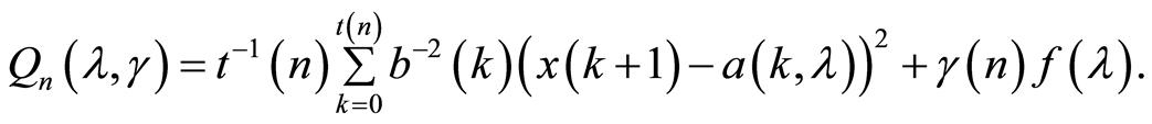 (2)
(2)
Here ,
,  ,
,  ,
,  is a real-valued function of the parameter
 .
.
With ,
,  , the functional (2) is an ordinary LS criterion which is constructed with the sample volume of
 . The sequential design for confidence estimation of the parameter
  will be regarded as a pair
  where
where

and  is a Markov moment relative to the family
  such that
 .
.
Let us consider the closed interval . It is obvious that
 , and we will use the
  as a confidence interval for the value of
 . Let
. Let  be u-neighbourhood of the interval
 ,
, . The properties of the sequential design
  are described by the following:
Theorem 1. Assume that the following statements are true:
1) For some  stochastic functions
 ,
,  are continuously differentiable in the neighbourhood
  and function
  is continuous on the
 .
.
2) 
3) For every ,
,  it is almost sure that a sequence of stochastic functions
converges on the .
.
4) If  then
then .
.
5) 
6) .
.
7) There exists a known constant .
.
8) .
.
Then for any  the following assertions hold true:
1) .
.
2) .
.
Remarks. The sequences ,
,  are parameters of the estimation procedure. In order to meet the condition 7, the sequences
 ,
,  may be definite, for example, in the form of
 ,
,  , where
 , [a]-integral part of the а,
 . Indeed

Proof of the Theorem 1. The proof is based on the following statements.
Lemma 1. [1] Let us assume that for a numeric sequence  and a sequence of the continuous on the compact K functions
  the following conditions are met:
1) If  the series
  converges.
2) If  the series
  converges uniformly in
 .
.
3) .
.
Then  converges uniformly in
 .
.
Lemma 2. [16] Let  be a sequence of continuous on the compact K stochastic functions for which the following conditions are met:
1) With every  a sequence
  is consistent with a nondecreasing flow of
  -subalgebras
2) If  the sequence
  converges uniformly on the
  and limiting function has the unique minimum in the point
 .
.
3) Then there exists a sequence of the random values  consistent with a nondecreasing flow of
  subalgebras
  and such that

Here  is the norm of the space in which the compact K is embedded.
Lemma 3. [17] Let the  is a stochastic and continuous on the interval
  function and for some constant
  the following conditions are met:

Then a constant B exists and for it the following assertion is true:
 .
.
This lemma is a corollary of the Theorem 19 [18] .
Lemma 4. Let us assume that the real function  and stochastic functions
 ,
,  in the (1) are continuous on the interval
 . If the conditions 2 - 4 and 7 of the Theorem 1 hold true, then we have

Proof on the Lemma 4. Consider the following representation:
From condition 2 of the theorem it follows that  is a square integrable martingale. From condition 2 of the Theorem 1 we have:
 a.s.
a.s.
Further using the strong law of large numbers for square integrable martingales [17] we have
 (3)
(3)
For every  let us say that
 .
.
It follows from conditions 2 and 8 of the Theorem 1 for the square integrable martingale  that the following assertion is true

and using the strong law of large numbers for square integrable martingales we have:
 . (4)
. (4)
From (3), (4) and condition 3 of the Theorem 1 and assertion of the Lemma 1 it follows that
 (5)
(5)
is realized uniformly in .
.
Further, using (1) and (2) we have:
Taking into account that  if
if ,
,  and (3), (5) as well as conditions 3, 4 of the Theorem 1, the following assertions hold true:
• If , series
  converges uniformly in
  almost sure.
• The limiting function of the series  have the unique minimum in the point
 .
.
From here and from assertion of the Lemma 2 we have

Hence, the Lemma 4 is proven. 
Let us get back to the proof of the Theorem 1. The  and
and  are strongly consistent estimates of the parameter
  (it follow from the Lemma 3). From here and from the continuity of the function
  is succeed
 .
.
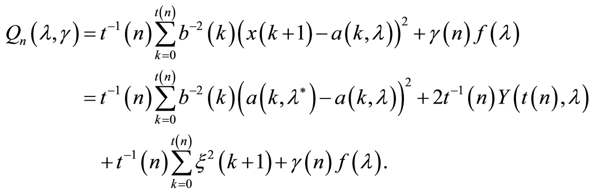
Using (2), we can see that
 (6)
(6)
Consider the set
 (7)
(7)
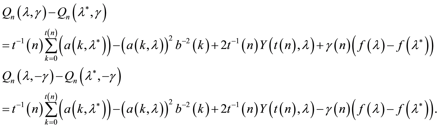
Taking into account that on the set (7) the following inequalities hold true
from (6) it follows that on the same set the following conclusions are true, too:
 (8)
(8)
By definition, the estimates  and
and  are the minimum points of the functions
  and
and , respectively, we have

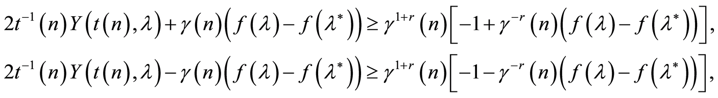
Using (8) we can assume that on the set (7) the following inequalities are true:
 (9)
(9)
Let us set the upper bound of the probability of the event (7) not happening:
 (10)
(10)
From the conditions 1, 2, 5 of the Theorem 1, the function  has the following properties:
 ,
,

Using this property (10) and assertion of the Lemma 3 we have
 . (11)
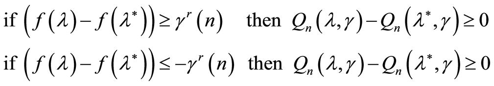
Using (9), (11) and condition 6, 7 of the Theorem 1 we can write that
The Theorem 1 is proven. 
Note. From Lemma 4 it follows that asymptotically the estimates of  represent usual estimates of the least squares.
4. Practical Example
Let us consider the problem of estimating the seawater absorption coefficient of the sonar signals in shallow water when sensors of a C-OTDR monitoring system are used for measurements. The fiber-optic sensor (FOS) of the C-OTDR monitoring system is laid on the sea bottom; it is an ordinary monomode fiber-optic line stowed inside of a special hygroscopic cable. At the logical level the entire length of this cable is split into equal portions duration of ~5 m. Each of these sections is called a logical C-OTDR channel or DAS (distributed acoustic sensor). Each DAS is able to measure the vibration of the hydrosphere which appeared in the area of its sensitivity. In fact, FOS consists of a huge number of vibration sensitive sensors successively arranged along the cable. A source of the hydroacoustic emissions (SHdE) emits a pulsed narrowband signal at a predetermined frequency. The coordinates of the SHdE are given. Therefore the angle of incidence of the hydroacoustic waves on FOS is also known. We denote this angle as . When the wave reaches the DAS system, the appropriate signal is fixed on N sensors (DAS) at successive times
  . Let’s denote the moment when the signal reaches the sensor as n (n is both the sensor’s number and the moment’s number). The signal goes through a group of sensors one by one as it moves at a particular speed. Thus, it reaches sensor 1 at the moment 1, sensor 2 at the moment 2 etc. The distribution of energy from the emitting source at each of the N sensors, at moments
  is described by the following equation:

Here  is the observed value of the signal energy in the n-th sensor at time n;
 —a noise component at moment
 , which appear due to the influence of the dispersing medium, and
 ,
,  ,
, ;
;  is a scalar function that describes the absorption of the elastic vibrations, this function depends on following parameters: water temperature T; value
 , where
  is the distance between the sensor number n and the sensor number
 ; n-sensor number; f-frequency of the SHdE. The function
  has the following simple form:
 . Here, the constant D is given and depends on the bottom and volume scattering. Function
  is a seawater absorption coefficient, which represents the basic interest for us. In turn, this function depends on an unknown parameter T (water temperature) and a given parameter f (frequency radiation of the SHdE). Observing
 , it is necessary to construct a confidence interval with fixed size for the seawater absorption coefficient
  by means of the sequential procedure which was suggested in the Section 3 of this paper. Parameters f, S, C are given. Experimental data (observations) was obtained for a depth of 50 m. The number of channels of the C-OTDR-system is 4000. Water temperature T at a depth of 50 m was considered a priori unknown and subject to estimation during the experiment. Thus, a primary purpose of the experiment was to estimate of the absorption coefficient of sea water
 , which depends nonlinearly on temperature T. In other words, the task was a interval estimation of the nonlinear function of the unknown parameter by dependent data
 . Table 1 shows the estimation results of the absorption coefficient values at different sensing frequencies
  and temperature
  with
with .
.
Here the “point estimates” were calculated by alternative methods. The temperature on the depth 50 m was determined by specialized sensors which were placed under water during the experiment for additional control. Once again, we point out that in the process of interval estimation , the water temperature T was considered unknown. The column “Required width of the confidence interval” contains information about a priori given size of the confidence interval for
  which we wish to get results for. The column “Average observation time” contains the average number of observation which had to be used to achieve the required width of the confidence interval in the sequential procedure. The content of this table shows that achieved results are practically acceptable.
5. Conclusions Remarks
In this paper we investigated some non-asymptotic properties of the modified least squares estimates for the non-linear function  by observations that nonlinearly depend on the parameter
 . The solution was found by sequence analysis. The obtained confidence region is valid for a finite number of data points when the distributions of the observations are unknown. If
 , the suggested method allows us to construct a confidence interval with fixed size for non-known parameter
 . The results of the practical application showed efficiency of the proposed approach.

Table 1 .Estimation results of the absorption coefficient.
Acknowledgements
This investigation has been produced under the project “Development of a remote monitoring system to protect backbone communications infrastructure, oil and gas pipelines and other extended objects (project code name— XY)”, financed under the project “Technology commercialization”, supported by the World Bank and the Government of the Republic of Kazakhstan.