1. Introduction
The Riemanean geometry is the study of curved surfaces. One might have a cylinder, or a sphere. For instance, one can use a cardboard paper towel roll to study a cylinder and a globe to study a sphere. In such spaces, the shortest curve between any pair of mass points on such curved surface is called a minimal geodesic or geodesic. One can find a geodesic between two mass points by stretching a rubber band between them. The first thing that will be noticed is that sometimes there is more than one minimal geodesic between two mass points. For instance, there are many minimal geodesics between the north and south poles of a sphere. This leads to derive more generalized formulas, which are true in the Euclidean space. Therefore, one of our main concern in this work is to motivate researcher for finding exact formulas for computing Barycenters on non-Euclidean spaces, namely on manifolds. In [1] , the authors suggest an estimation of the so-called Riemannean Barycenters. For a use in the same context, we refer for instance to [2] . Where, in [3] Riemannian means were presented as solution of variational problems. We think that for special case, for instance smooth manifolds, we could derive similar formulas to the Euclidean case, define and study interesting properties of Riemannean Barycenters.
In this work, we begin by setting out some basic theory of the geodesic of the unit circle as one dimensional manifold, we define the multiple Barycenters and compute it for some special cases. For more details, we refer to [4] -[6] .
Let I be an interval of real numbers. Then, a curve γ is a continuous mapping given as  where
where  is a smooth Riemannean manifold. The curve γ is said to be simple if it is injective. If I is a closed bounded interval [a, b], we also allow the possibility
  (this convention makes it possible to talk about closed simple curve). If
  for some
  (other than the extremities of I), then
  is called a double (or multiple) point of the curve. A curve γ is said to be closed or a loop if I = [a, b] and if
 . A closed curve is thus a continuous mapping of the circle. Let x, y are two points of
  subset of
 . If γ is a curve such that
 ,
,  and
and 
 we said that γ is a connection between x and y. We define
  the set of all connections between x and y on
 . Let x, y be two mass points of
 . The geodesic is the minimum distance between x and y on
  (or the shortest path), denoted by
 , which is given by
 . We say that X is a geodesic space if for any pair
  there is a minimal geodesic from x to y and this is given as a minimal of
 , where
  is a curve joining x and y. Let two points
 . The geodesic (shortest path) between the two points x and y is given by
 , where
 , is the scalar product on
 . The shortest geodesic (which is a metric on
  that joins two non antipodal points. The geodesic distance between the two points is precisely equal to α. A midpoint m of two masses on
  is defined
  where g is a geodesic on
 . For more details, we refer to [7] -[9] .
Example 1. Consider the following examples on the unit circle:
1) Each point on  is midpoint of itself
2) The midpoint of  and
and  is the unique point
 , therefore

3) Observe that even if  for
for . The fact that
  is not a geodesic between x and y.
4) The midpoint on  is not unique: Consider
  (north pole) and
  (south pole),
 .
.
2. Barycenters on 
The arithmetic mean of a finite set of mass points  the Euclidean space
 . is the unique point x that minimizes the sum of the squared distances to the given mass point, that is
 , where d(·,·)
is an Euclidean distance in . The point realizing the minimum of the function
  is called also Barycenter of the set of mass points
 . In this section we would like to extend this definition to a smooth Riemannean manifold
 , and for more information, we refer to [1] [3] .
Definition 1. The Barycenter of the set of mass points  subset
  with weighs
  (respectively) is the mass point minimizing the following functional (Energy function):
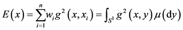
where g(·,·) is the geodesic in  and μ is the distribution in the continuous case.
Lemma 1. Let  and
and  are two mass points with weights
  and
and , such that
with ,
,  and
and . If
. If  is the geodesic Barycenter of
  in
in , then there exists
  such that
Proof. We prove that the geodesic Barycenter of two mass points is a mass point contained on the shortest path. We have

Suppose that  is not element of
 . There exists
  such that

it follows

( is not element of
 ). It implies

In fact, the point  satisfies the minimal and the following equality
Lemma 2. Let two mass points  with weights
  and
and  respectively. If for all
 are unique, then the geodesic Barycenter of
  is unique.
Proof. Suppose that the Barycenter is not unique, and denote by  and
and  solving the energy functional. From Lemma 1, we know that the geodesic Barycenter is contained on the shortest path between
 , it means

 there exists two geodesics connecting
 , this contradicts the uniqueness of the geodesic.
Definition 2. Let an oriented unit circle with origin , and a subset of mass points points
 . We denote by
  the number of all geodesics, their corresponding curves contain the origin
  where
where 
3. Geodesic Multiple Barycenters on 
The existence of Barycenters on  interpreted as one dimensional Riemannean space does assure it uniqueness. In this section, we give a general condition of the existence of a geodesic multiple Barycenter on
 .
.
Definition 3. (Geodesic Multiple Barycenter). We said that a set of mass points have a multiple Barycenter if the solution of the energy function is not unique.
Example 2.
1) The Barycenter of the north and south poles is not unique i.e. 0 and .
.
2) We examine a simple example on the unit circle. Compute the Barycenter of four mass points
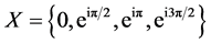


Define 
It implies

Differentiations with respect to z
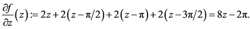
1)  with
with :
:
From  it follows
  and
and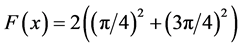 .
.
2)  with
with :
:
From  it follows
  and
and .
.
3)  with
with :
:
From  it follows
  and
and .
.
4)  with
with :
:
From  it follows
  and
and .
.
We conclude that  4 are Barycenters of the set X.
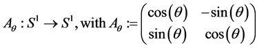
Definition 4. (Symmetry propriety SP). Let  be a mass distribution on the unit circle. The map
  is called a symmetry of
  if: σ is an isometry and
Example 3. , for which
  satisfies the map
the symmetry propriety.
The mass distribution is defined on two points
 ,
,  on
on  such that

It is clear that for ,
, . If the distribution is defined over the set of equidistant masses
 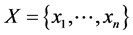 then for
  with
with  -rotation on the unit circle, with a supplementary propriety that
  such that
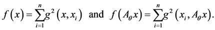
Figure 1 shows some example of symmetry mass points on  (From left to right) On the first figure, we have two mass points antipodal, the first on (1, 0) Cartesian coordinate and the second in (0, 1). The second, third and fourth show other types of semmetries.
Theorem 1 (Multiple Barycenter). Let  on
on  be a set of n mass points. If there exists a symmetry map Aθ, then x admits a multiple Barycenter.
Proof. For n = 2 and 
 is the symmetry map such that
 . Then for all
 hold,
hold,

It follows from our assumptions that  for all
  It is clear that
  for all
 and if for all
  is a Barycenter of for all
  then
then  is too. In this case we have double Barycenters. Now suppose that n > 2. Then, for all
  we have
Moreover

Thus

Lemma 3. Under the same assumptions of Theorem 1. Let k be the number of the symmetry maps  in S1 which have the propriety
 , i.e. the distribution of the mass points is
  -invariant. The number of the multiple Barycenters is k + 1.
Proof. The proof is left to the reader.
Figure 2 contains three, four, five, six, eight and nine mass points satisfying the symmetry property and non necessary with same weights. The geodesic between two arbitrary and successive mass points is constant. I each of the figures our code generates all possible Barycentes so-called multiple Barycenters.
Figure 3 shows the uniqueness of the Barycenter on  in the case of four masses without symmetry property.
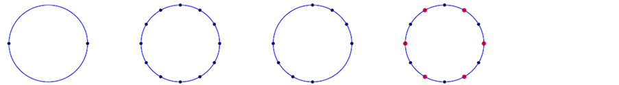
Figure 1. Examples of symmetry masses distribution on S1.
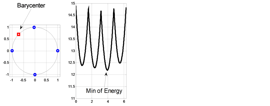
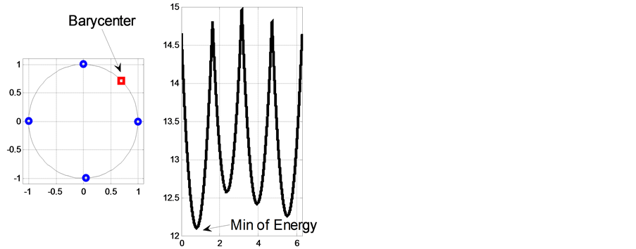
Figure 3. Case of non-symmetry on S1 (uniqueness of the Barycenter. (small perturbation of the north and south poles respectively.
4. Concluding Remarks
As consequence of the non-uniqueness geodesic between two arbitrary mass points, we have presented an example on the notion of multiple Barycenters. Moreover, we have derived some properties similarly to the Euclidean space. We believe that more interesting cases are to construct significant formulas for arbitrary manifolds.
Acknowledgements
The authors would like to dedicate this work to Dr. Musaed Al-Subhi Rahimaho Allah.
NOTES
*Corresponding author.