Optimal Expected Utility of Wealth for Two Dependent Classes of Insurance Business ()
1. Introduction
The classical Cramer-Lundberg risk model assumes that the number of claims up to time t is independent of the claim size  and the claim sizes are independent and identically distributed. However, the independence assumption can be restrictive in practical applications. Several authors have therefore suggested models where the risks dependence is assumed. Within this models, we distinguish between risk models with dependence among claim size and among inter-occurrence time (see [1-5]) and risk models that consider aggregate claims amount processes generated by correlated classes of insurance business (see [6-13]). In [14] a wide set of dependent risk processes involving particular classes is presented with references therein. In some cases, the authors consider reinsurance contracts (see [9,10]) to improve the risk situation to which the company is subjected. In particular, [10] suggests an unlimited Excess of Loss reinsurance and maximizes the expected utility of the wealth of the insurer or the adjustment coefficient. In this paper, we consider a risk model involving two dependent classes of insurance business and a limited Excess of Loss reinsurance with the aim to maximize the expected utility of the first insurer wealth, having the retention limits as decision variables. The paper is organized as follows. Section 2 presents the risk model and the reinsurance contract. In Section 3 the maximization problem is proposed and in Section 4 the solution is discussed.
2. The Model
We consider a risk model involving two dependent classes of insurance business. Let  be the claim size random variables for the first class with common distribution function
  and let
  be those for the second class with common distribution function
 . We assume that
  and
and  have continuous and positive first derivative, with
  if
if  Their expected values are denoted by
  respectively. Then, the aggregate claims amount process generated from the two classes of business, in a given period of time, is
  with
with
 , (1)
, (1)
where  is the number of claims, for classes
 , in the given period of time.
We assume that  and
and  are independent, and they are independent of
  and
and . The claim number processes are correlated by means of the following relationships (see [10]):
 (2)
(2)
where  and K are independent Poisson random variables with parameters
  and
and , respectively.
As usual, we define the surplus process in the given period of time:
 (3)
(3)
where , is the insurance premium of risk i and u is the value of the surplus at the beginning of the time period.
We assume the following exponential utility function:
 (4)
(4)
then, in the absence of reinsurance, the expected utility of wealth is
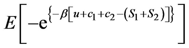 (5)
(5)
We instead assume that the first insurer concludes an Excess of Loss (XL) reinsurance contract limited by , with retention limits
 , for the respective classes of insurance business. In [10], an unlimited XL reinsurance is considered.
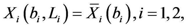
In the following, we will consider the variables , identically distributed to
 . In practical, XL reinsurance contracts with retention limit
  are limited by some constant
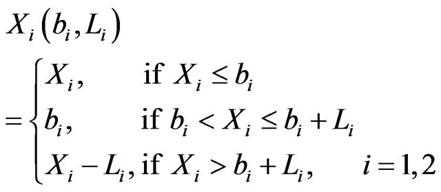
 , which leads to the following division of claim size
 .
.
The reinsurer pays 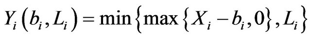
and the first insurer pays what is left: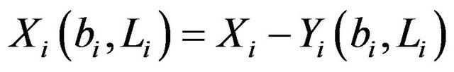 , (see [15]). That is:
 (6)
(6)
and
 (7)
(7)
Observe that if  the limited XL reinsurance becomes unlimited. We fix
  with
with , for the two classes of insurance business, respectively, and we make use of the retention limits
 , as decision variables. We refer to (6) and (7) and we set
 (8)
(8)
identically distributed to the j-th payment of the reinsurer  and
and
 (9)
(9)
identically distributed to the j-th payment of the first insurer .
.
Then, the aggregate claims amount process for the insurer generated from the two classes of business after reinsurance, in a given period of time, is  with
with
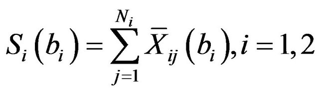 . (10)
As usually, the reinsurance premiums are evaluated as follows:
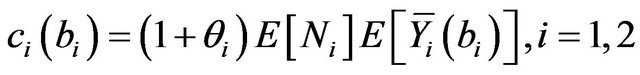 where
where , is the corresponding safety loading. We therefore have
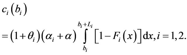 (11)
(11)
Then, after reinsurance, the surplus process in the given period of time is
 (12)
(12)
and the expected utility is
 (13)
(13)
In the following Section, we will take the problem of the maximization of the wealth expected utility, having the retention limits , as decision variables.
3. The Problem
As already mentioned, our problem is to find the pair , with
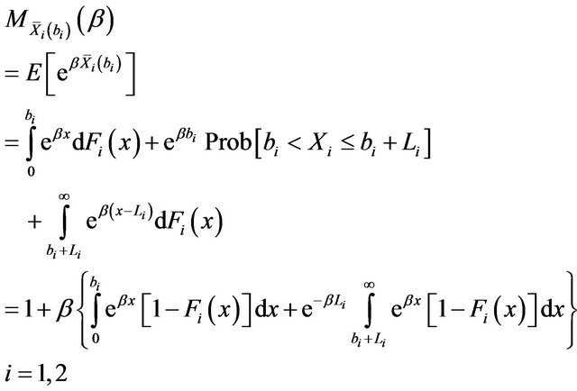
 , that maximizes (13). We observe that from the moment generating function of the bivariate Poisson distribution (see [10,16]) it follows that
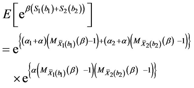 (14)
(14)
where we assume that the moment generating function
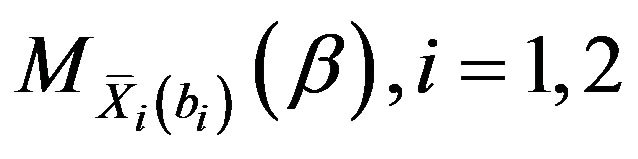 , exists. In particular, we assume that the variables
  have a limited distribution or that the following relationship is true:
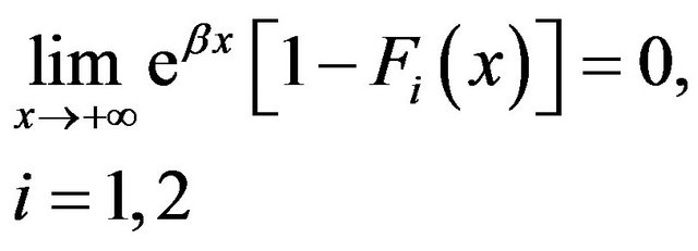 (15)
(15)
It therefore results
(16)
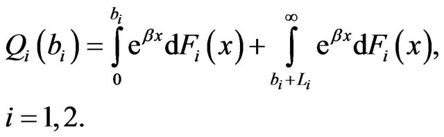
We put:
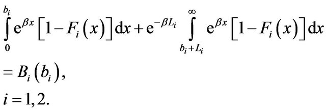 (17)
(17)
and we straightaway observe that
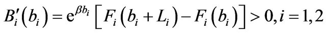 (18)
(18)
since it is  and
and 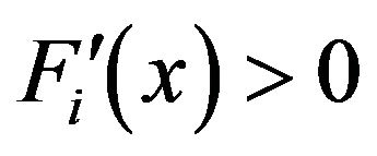 by assumption.
Because of (14), (16) and (18), (13) can be written as
 (19)
(19)
that is, putting
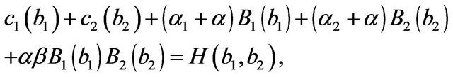
we have
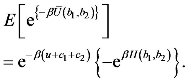 (20)
(20)
Therefore, maximizing (13) is equivalent to minimizing  it follows that, since
 , our problem consists of
 (21)
(21)
We proceed in a similar way to that followed in [10]. The Kuhn-Tucker conditions for the P problem are
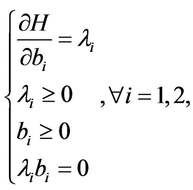 (22)
(22)
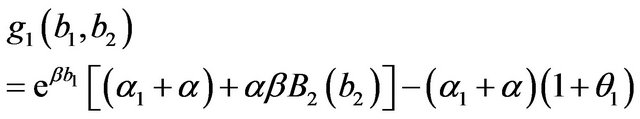
where, remembering (11) and (18):
 (23)
(23)
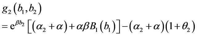
and
 (24)
(24)
Let us start by proving the following theorem.
Theorem 1.
The Hessian matrix of  is negative definite, whenever the gradient is null.
Proof. Considering (23) and (24), it results
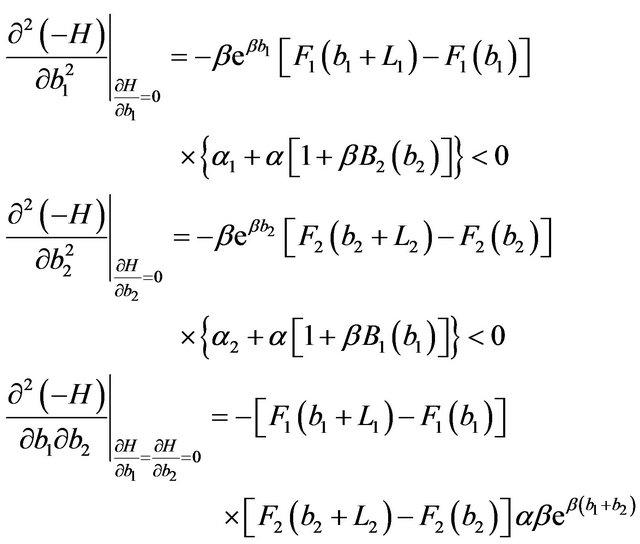
and
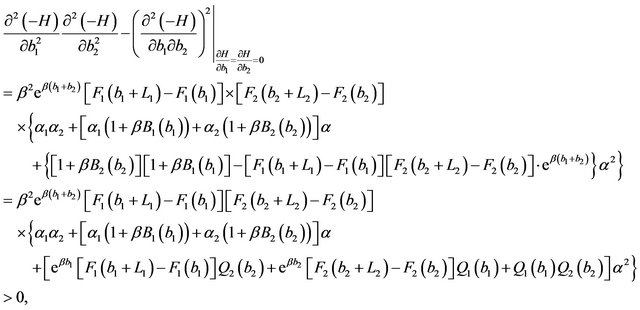
where
4. The Khun-Tucker Conditions
We look for the points  that fulfill the KuhnTucker conditions. To this purpose, we put
 (25)
(25)
 (26)
(26)
 (27)
(27)
and we prove the following theorem where  and
and , are defined by (25), (26) and (27), respectively.
Theorem 2.
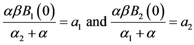
1) The point  satisfies the system (22) if and only if it is
 (28)
(28)
2) The point , with
 , satisfies the system
(22) if and only if it is
 (29)
(29)
3) The point , with
 , satisfies the system
(22) if and only if it is
 (30)
(30)
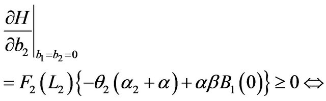
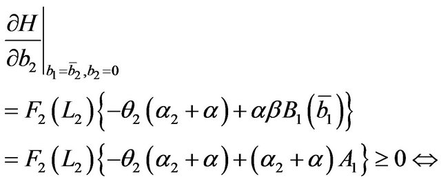
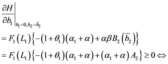
4) If it is
 (31)
(31)
and it is
 (32)
(32)
or
 (32')
(32')
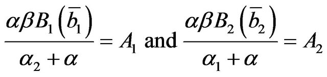
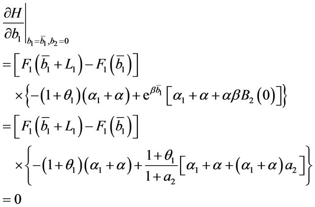
then it exists the point , with
 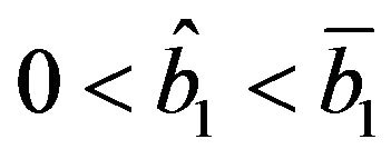 and
and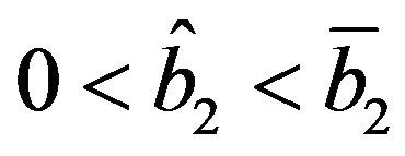 , satisfying the system (22), and it is
 (33)
(33)
Proof.
1) It results

the first of (28) holds and
the second of (28) holds.
2) We recall that  is defined by (26). From (29) it follows that
  the first of (29) holds.
Furthermore, remembering (25) and (26),
and, remembering (27)
the second of (29) holds.
3) We recall that  is defined by (26). From (29) it follows that
  the second of (30) holds.
Furthermore, remembering (25) and (26),

and, remembering (27)
the first of (30) holds.
4) Because of (31) it results
 (34)
(34)
We put
and
and we note that it results
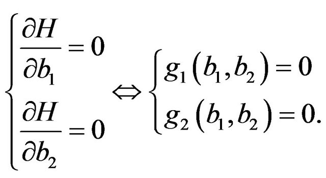 (35)
(35)
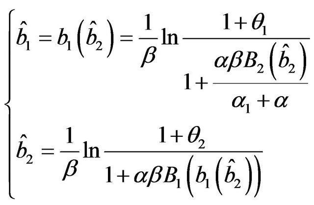
We solve the system (35). We have:
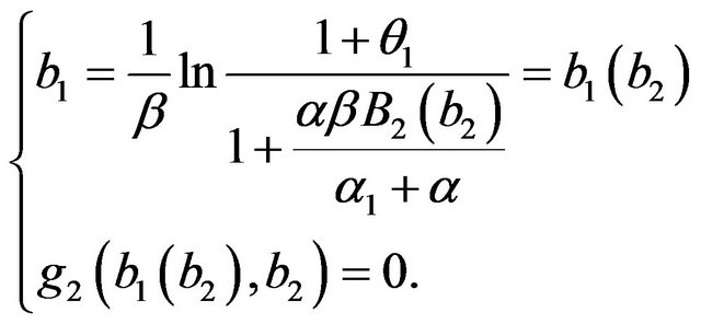 (36)
(36)
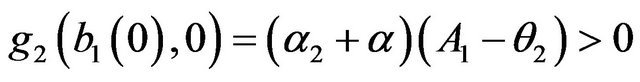
To solve the equation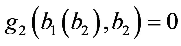 , we make use of a similar procedure to that in [10]. We note that g2 is a continuous function of
  and that, by (34), it results
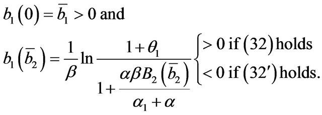
If (32) holds, remembering (27) and (25), and being  an increasing function, it results
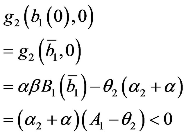
and
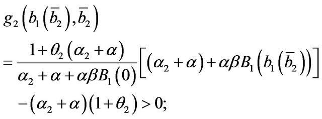
it therefore exists , satisfying the second of (36). Substituting
  in (36), it results
 (37)
(37)
with, by (31) and (32), since  is an increasing function:
 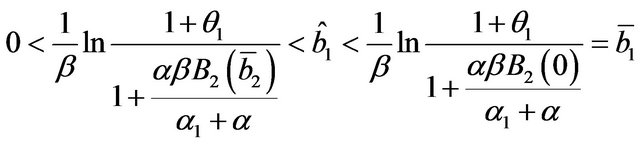 (38)
(38)
therefore,  satisfying (33) fulfills the system (22).
Similarly, if (32’) holds, remembering (27) and (25), and being  an increasing function, it results
and

it therefore exists , satisfying the second of (36). Substituting
  in (36) we obtain (37), (38) and the point
  fulfilling the system (22).