1. Introduction
Mathematical epidemiology plays an important role in our society. Epidemic models to represent the interaction of different individuals by linear and nonlinear incidence have been discussed by many authors [1-3]. Literature of SIR diseases transmission model is quite large see [4-6], where S represents the number of individuals that are susceptible to infection, I represents the number of individuals that are infectious and R denotes the number of individuals that have recovered. The SIR epidemic models are used in epidemiology to compute the amount of susceptible, infected and recovered people in a population. These models are also used to explain the dynamics of people in a community who need medical attention during an epidemic. However, it is important to note that these epidemic models do not work with all diseases. For the SIR model to be appropriate, once a person has recovered from the disease, they would receive lifelong immunity. But if a person was infected but is not infectious then someone need to modify the SIR epidemic model by including exposed class. The mathematical representation of SIR epidemic model consisting of three coupled ordinary equations which represents the dynamics of susceptible, infected and recovered individuals, respectively is given by

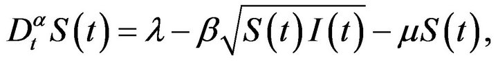
where λ is the constant birth rate, μ is the natural death rate,  is the fraction of infected individuals who leave the infected class per unit time, β is the rate of production of new infected individuals, and f(S, I) is a function relating the rate of conversion of the susceptible population to the infected population. Mickens [7] introduced first time the square root interaction term in the SIR-model is given by
 (1)
(1)
 (2)
(2)
 (3)
(3)
With

The total population is 
So we obtain by adding all equations of above system
 (4)
(4)
Differential equations of fractional order have been the focus of many studies due to their frequent appearance in different applications in fluid mechanics, biology, physics, epidemiology and engineering. Recently, a large amount of literatures developed concerning the application of fractional differential equations in nonlinear dynamics [8-10]. The differential equations with fractional order have recently proved to be valuable tools to the modeling of many physical phenomena. This is because of the fact that the realistic modeling of a physical phenomenon does not depend only on the instant time, but also on the history of the previous time which can also be successfully achieved by using fractional calculus. The reason of using fractional order differential equations is that fractional order derivatives are naturally related to systems with memory which exists in most biological systems. Also they are closely related to fractals which are abundant in biological systems. As fractional calculus is the generalization of the ordinary differentiation and integration to non-integer and complex order. Also because of fractional order derivatives many authors established new models in different fields. In this paper, we consider a square root interaction in the SIR-model presented by Mickens [7] in fractional order. First we show the positive solution of square root interaction in the SIR epidemic model in fractional order. Then, we show the local stability of the epidemic model with fractional order. Finally, we compare our numerical results with nonstandard numerical method and fourth order Runge-Kutta method.
This paper is organized as: In Section 2, we present formulation of the model with some basic definitions and notations related to this work. In Section 3, we show the non-negative solution and uniqueness of the model. In Section 4, the local stability of the model is presented. In Section 5, the numerical simulations are presented graphically. Finally, we give conclusion.
2. Formulation of Model with Preliminaries
In this section, we present the SIR-model for which the interaction term is the square root of the susceptible and infected individuals in the form of fractional order differential equations. The new system is described by the following set of fractional order differential equations:
 (5)
(5)
 (6)
(6)
 (7)
(7)
 (8)
(8)
Here  is fractional derivative in the Caputo sense and
  is a parameter describing the order of the fractional time-derivative with
 . For
. For  the system will be reduced to ordinary differential equations. This kind of fractional differential equations is the generalizations of ordinary differential equations. Now we give some basic definitions related to this work and can be found in fractional calculus see for example [11-15].
Definition 1 A function  is said to be in the space
  if it can be written as
  for some
  where
where  is continuous in
 , and it is said to be in the space
  if
if .
.
Definition 2 The Riemann-Liouville integral operator of order  with
with  is defined as
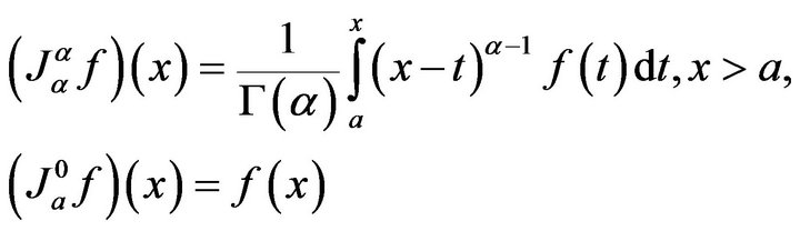
Properties of the above operator can be found in [11].
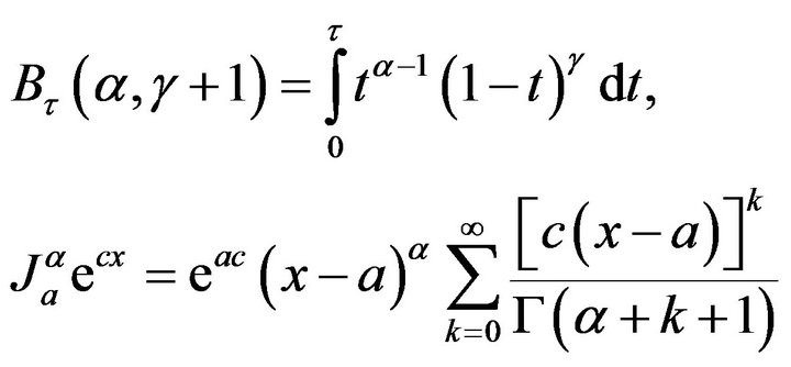
Definition 3 For  and
and  we have

where  is the incomplete beta function which is defined as
The Riemann-Liouville derivative has certain disadvantages when trying to model real-world phenomena with fractional differential equations.
Definition 4 The Caputo fractional derivative of  of order
  with
with  is defined as
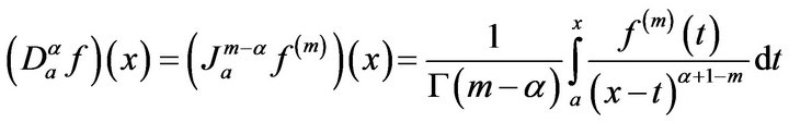 for
for 
The fractional derivative was investigated by many authors, for  and
and , we have
 .
.
The definition of fractional derivative involves an integration which is non-local operator (as it is defined on an interval) so fractional derivative is a non-local operator. In other word, calculating time-fractional derivative of a function  at some
  time requires all the previous history, i.e. all
  from
from  to
to .
.
3. Non-Negative Solutions
In this section, we show the positivity of the system. We first consider
and
 .
.
In order to prove the theorem about non-negative solutions, we need to state the following Lemma [9].
Lemma 3.1. (Generalized Mean Value Theorem) Let  and
and  for
for . Then we have
 with
with , for all
Remark 3.2. Suppose and
and
 for
for . It is clear from Lemma 3.1 that if
  for all
 , then the function f is non-decreasing, and if
  for all
 , then the function f is non-increasing.
Theorem 3.3. There is a unique solution for the initial value problem given by (5)-(8), and the solution remains in .
.
Proof. The existence and uniqueness of the solution of (5)-(8), in  can be obtained from [5, Theorem 3.1 and Remark 3.2]. We need to show that the domain
  is positively invariant. Since

On each hyperplane bounding the non-negative orthant, the vector field points into .
.
4. Local Stability Analysis of Model
The system of ODE’s given by (1)-(3) has a unique non-trivial solution. By setting the right hand side of the Equations (1)-(3) equal to zero, we get

All the parameters are taken to be positive, then  are positive. For the unique positive equilibria the Jacobian matrix at this fixed point is

here

The eigen values  are given by
 where I3 is the unit matrix of order 3 × 3. By evaluating this determinant we obtain the following equation
 (9)
(9)
It is clear that λ1 = −μ is negative. For others roots we can write
 (10)
(10)
Let the remaining roots of this equation are λ2 and λ3, that satisfying the following relations
 (11)
(11)
From Equation (11) we conclude that:
1) If λ2 and λ3 are real, then both roots have same sign.
2) If λ2 and λ3 are real, then both roots are negative.
3) If λ2 and λ3 are complex, then λ2 = λ3 and the real parts are negative.
4) Thus, all the eigenvalues are negative or have negative real parts, and hence we conclude that this fixed point is located at  is locally stable.
5. The NSFD Scheme
In general, the non-standard finite difference rules, introduced by Mickens [7,16-19], do not lead to a discrete model for the unique solution of any dynamical system based on differential equations. First, we give the basic rules of nonstandard ordinary differential equations (ODEs) is given by

where  is the nonlinear term in the differential equation. Using the finite difference method we have
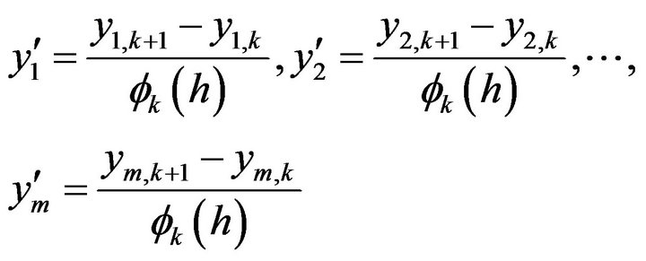
where  is a function of the step size h = Δt. The function
  have the following properties:
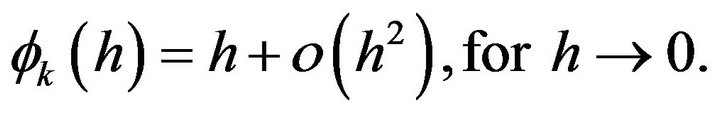 (12)
(12)
Examples of functions  that satisfy (12) are h,

Non-linear terms can in general be replaced by nonlocal discrete representations, for example

here 
The NSFD scheme for (1)-(4) system is shown as follows:
 (13)
(13)
Here

Now making the transformation of variables
 (14)
(14)
in the first equation of system (13), we obtain a quadratic equation for ,
,
 (15)
(15)
Note that our interest is calculating  which is based on the knowledge of
 , and then we used the transformation given in Equation (14). The solution for the quadratic Equation (15) is

Similarly, the remaining equations of the system (13) can be solved for the variables at the  time step:

6. Numerical Method and Simulation
In this section we find the numerical solutions. For numerical simulation, we use μ = 0.04,  = 0.03, β = 0.05 and λ = 1. For the effectiveness of the proposed algorithm which as an approximate tools for the solution of the nonlinear system of fractional differential Equations (1)-(4). Figures 1-4 show the approximate solutions obtained using ODE45 and classical RK4 method of S(t), I(t), R(t) and N(t) when α = 1. Figures 5-8 show the

Figure 1. The plot represents the susceptible individuals.
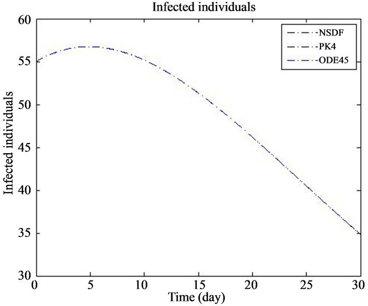
Figure 2. The plot represents the infected individuals.
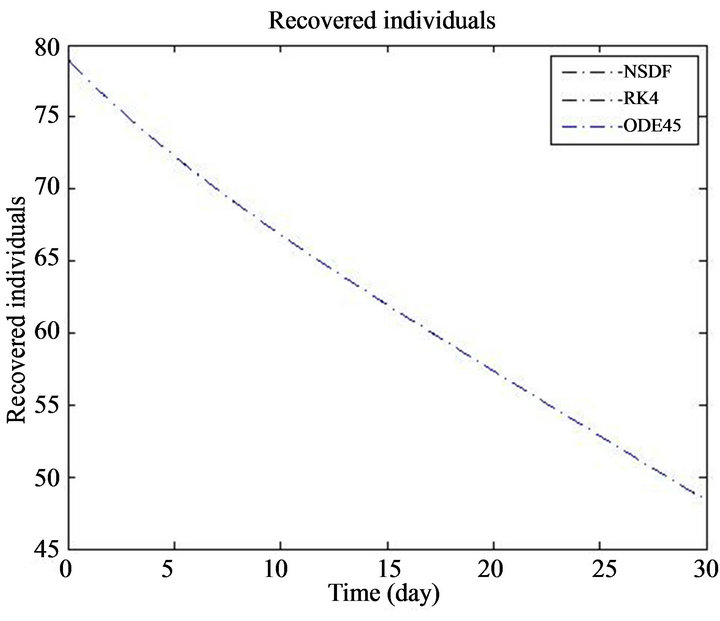
Figure 3. The plot represents the recovered individuals.

Figure 4. The plot represents the total population.

Figure 5. The plot represents the susceptible individuals for different values of α.

Figure 6. The plot represents the infected individuals for different values of α.

Figure 7. The plot represents the recovered individuals for different values of α.
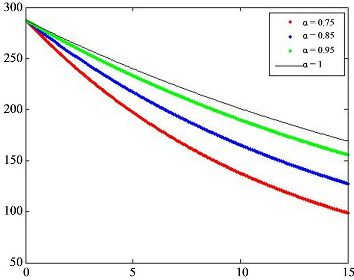
Figure 8. The plot represents the total population for different values of α.
approximate solutions of S(t), I(t), R(t) and N(t) for α = 0.75, 0.85, 0.95, 1.
7. Conclusion
In this paper, we introduced fractional derivatives in the SIR epidemic model with square root interaction of the susceptible and infected individuals. First the non-negative solution of the model in fractional order is presented. Then the local stability analysis of the model in fractional order is presented. Finally, the general solutions were also discussed and a discrete-time, finite difference scheme is constructed using the nonstandard finite difference (NSFD) method.
8. Acknowledgements
This study was founded by the National Fisheries Research and Development Institute (RP-2012-FR-040).
NOTES