1. Introduction
A study of the thermophysical properties as a function of pressure and temperature in a homologous series of chemical compounds is of great interest not only for industrial applications for example, in the petroleum industry, but also for fundamental aspects for understanding the influence of the chain length of the components on the liquid structure and then developing models for an accurate representation of the liquid state. With this aim in mind, a research program of thermal pressure coefficients (TPC) measurements under pressure on most paraffins between decane and triacontane was initiated as a part of a project on crude oil characterization [1-3].
One of the most difficult problems within the context of the thermodynamics lies in the shortage for experimental data for some basic quantities such as thermal pressure coefficients (TPC) which are tabulated for extremely narrow temperature ranges, normally around the ambient temperature for several types of liquids. Furthermore, the measurements of the thermal pressure coefficients made by different researchers often reveal systematic differences between their estimates [4,5].
The idea has been presented a simple method that use to calculate thermal pressure coefficient directly in place of using equations of state to analysis experimental pVT data [6-8]. The equation of state described in papers is explicit in Helmholtz energy  with the two independent variables density
  and
and . At a given temperature, the thermal pressure coefficient can be determined by Helmholtz energy [9-15].
Another work has led to try to establish a correlation function for the accurate calculation of the thermal pressure coefficients for different fluids over a wide temperature and pressure ranges. The most straightforward way to derive the thermal pressure coefficient is the calculation of thermal pressure coefficient with the use of the principle of corresponding states which covers wide temperature and pressure ranges. The principle of corresponding states calls for the reduced thermal pressure at a given reduced temperature and density to be the same for all fluids. This is true, since the corresponding-states approach is appropriate for conditions of low density in which the fluid molecules are far apart and thus have little interaction. Moreover, at low density, the gas behaves ideally and its thermal pressure coefficient is temperature independent and approaches  in the zero-density limit. However, as density increases, molecular interactions become increasingly important and the principle of corresponding states fails. The leading term of this correlation function is the thermal pressure coefficient of a perfect gas, which each gas obeys in the low density range. Using this condition it can predict the thermal pressure coefficient of different supercritical fluids and refrigerants up to densities
 . As mentioned before, as density increases, molecular interactions become increasingly important and the principle of corresponding states fails. It found out “empirically” that at high densities it is possible to apply the principle of corresponding states to different fluids according to the magnitude of their critical densities versus
  mol·dm–3 [16].
A general regularity was reported for pure dense fluids, namely testing literature results for pVT for pure dense fluids, according to which  is linear with respect to
  for each isotherm, where
  is the compression factor. This equation of state works very well for all types of dense fluids, for densities greater than the Boyle density but for temperatures below twice the Boyle temperature. The regularity was originally suggested on the basis of a simple lattice-type model applied to a Lennard-Jones (12,6) fluid. The purpose of this paper is to examine whether the regularity extends to calculation of the thermal pressure coefficients in liquid nPentadecane (C15), n-Heptadecane (C17), n-octadecane (C18) and n-nonadecane (C19) [17,18].
At present work, linear isotherm regularity has been used to calculate the thermal pressure coefficient. The purpose of this paper is to point out an expression for the thermal pressure coefficient of dense fluids using the linear isotherm regularity. In this article, in Section 1, we present a simple method that keeps first order temperature dependency of parameters in linear isotherm regularity versus inverse temperature. Then, the thermal pressure coefficient is calculated by linear isotherm regularity. In Section 2, temperature dependency of parameters in linear isotherm regularity has been developed to second order. In Section 3, temperature dependency of parameters in linear isotherm regularity has been developed to third order and then thermal pressure coefficient is calculated by linear isotherm regularity in each state.
2. Theory
A general regularity which was reported for pure dense fluids, according to which  is linear with respect to
 , each isotherm as,
 (1)
(1)
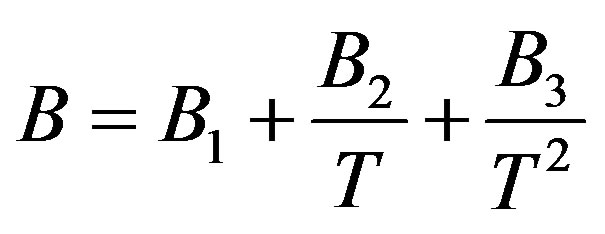
where  is the compression factor,
  is the molar density, and A and B are the temperaturedependent parameters.
 (2)
(2)
2.1. First Order Temperature Dependency of Parameters
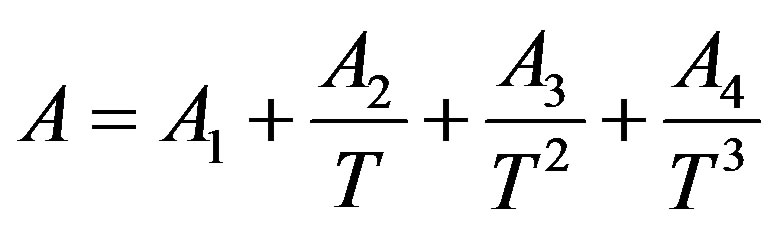
We first calculate pressure by linear isotherm regularity, and then use first order temperature dependency of parameters to get the final the thermal pressure coefficient for the dense fluid. Where
 (3)
(3)
 (4)
(4)
Here  and
and  are related to the intermolecular attractive and repulsive forces, respectively, while
  is related to the non-ideal thermal pressure and
  has its usual meaning.
In the present work, the starting point in the derivation is Equation (2). By substitution of Equation (3) and Equation (4) in Equation (2) we obtain the pressure for dense fluid.
 (5)
(5)
We first drive an expression for the thermal pressure coefficient using first order temperature dependency of parameters. The final result is 
 (6)
(6)
According to Equation (6), the experimental value of density and value of  from the Table 1 can be used to calculate the value of the thermal pressure coefficient.
For this purpose we have plotted  versus
  that intercept shows value of
 . Table 1 shows the
  values for four fluids of C15H32, C17H36, C18H38 and C19H40. Then we obtain the thermal pressure coefficient of C15H32, C17H36 , C18H38 and C19H40 dense fluids. C17H36 serve as our primary test fluids because of the abundance of available pVT data. Such calculations are similar to the other fluids examined. Because plots are subject to experimental error, we also show the coefficient of determination R2, which is simply the square of the correlation coefficient. Here R2 should be within 0.005 of unity for a straight line to be considered a good fit [4,18]. In result, the linear limit is estimated by a limit of
 . Thus, in according with the square of the correlation coefficient in Table 1, the thermal pressure coefficient using the LIR(0) model yields inaccurate results for the liquid phase. Also, this deviation exists significantly for the
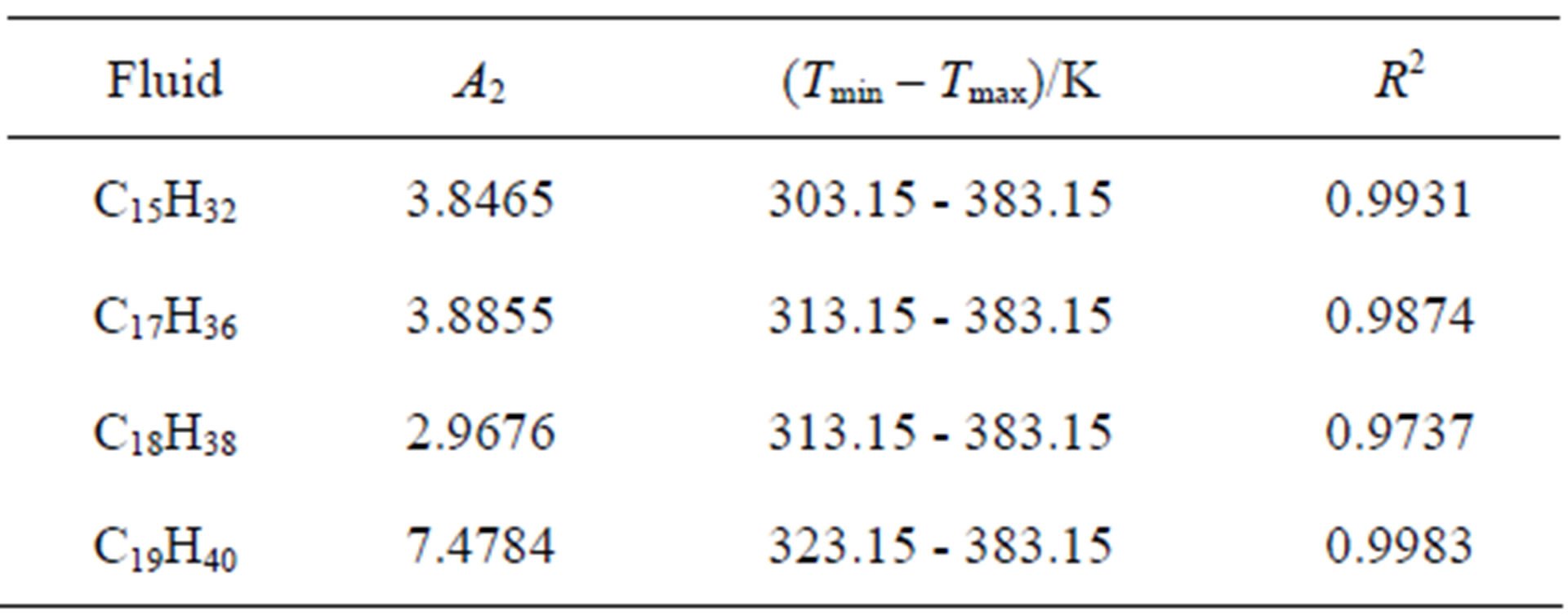
Table 1. The calculated values of A2 for different fluids using Equation (3) and the coefficient of determination (R2).
supercritical phase. Whereas, we predict that deviation concern to be inaccurate values of A2. For this purpose we have plotted A versus  that intercept shows value of
 . Figures 1(a) and (b) show plots of A and B versus inverse temperature for C17H36. It is clear that A and B versus inverse temperature are not first order.
2.2. Second Order Temperature Dependency of Parameters
In order to solve this problem, the linear isotherm regularity equation of state in the form of truncated temperature series of A and B parameters have been developed to second order for dense fluids. Figures 2(a) and (b) show plots of A and B parameters versus inverse temperature for C17H36 fluid. It is clear that A and B versus inverse temperature are second order. Thus, we obtain extended parameters A and B resulted in the second order equation, as
 (7)
(7)
 (8)
(8)
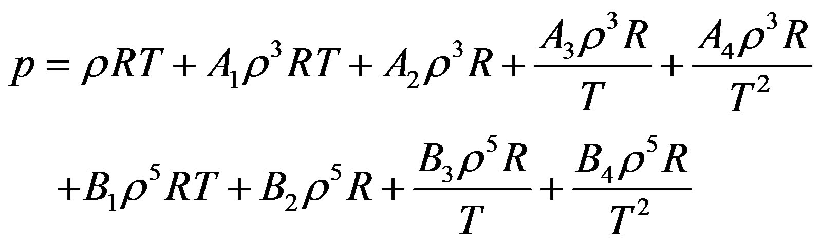
The starting point in the derivation is Equation (2) again. By substitution of Equations (7) and (8) in Equation (2) we obtain the pressure for dense fluid.
 (9)
(9)
First, second and third temperature coefficients and their temperature derivatives were calculated from this model and the final result is for the thermal pressure coefficient to form .
.
 (10)
(10)
As Equation (10) shows, that it is possible to calculate the thermal pressure coefficient at each density and temperature by knowing . For this purpose we
 1000*K/T(a)
  1000*K/T(b)
Figure 1. (a) Plot of A versus inverse temperature. The solid line is the linear fit to the A data points, for C17H36; (b) Plot of B versus inverse temperature. The solid line is the linear fit for C17H36 .
have plotted extending parameters of A and B versus  that intercept and coefficients show the values of
 that are given in Table 2.
2.3. Third Order Temperature Dependency of Parameters
In another step, we test to form of truncated temperature series of A and B parameters to third order (Figures 3(a) and (b)).
 1000*K/T(a)
  1000*K/T(b)
Figure 2. (a) Plot of A versus inverse temperature. The solid line is the linear fit to the A data points, for C17H36; (b) Plot of B versus inverse temperature. The solid line is the linear fit for C17H36 .
 1000*K/T(a)
  1000*K/T(b)
Figure 3. (a) Plot of A versus inverse temperature. The solid line is the linear fit to the A data points, for C17H36; (b) Plot of B versus inverse temperature. The solid line is the linear fit for C17H36.

Table 2. The calculated values of A1, A3, using Equation (7) and B1, B3, using Equation (8) for different fluids and the coefficient of determination (R2).
 (11)
(11)
 (12)
(12)
The starting point in the derivation is Equation (2) again. By substitution of Equations (11) and (12) in Equation (2) we obtain the pressure for dense fluid.
 (13)
(13)
The final result is for the thermal pressure coefficient to form .
.
 (14)
(14)
That based on Equation (14) to obtain the thermal pressure coefficient, it is necessary to determine values  that these values are given in Table 3.
3. Experimental Tests and Discussion
Specific experiments on heavy hydrocarbons to set up a base which can then be used to define new models specially adapted to these complex mixtures. With this aim in mind, an investigation was carried out on pure hydrocarbons with more than 16 carbon atoms, as hexadecane is the crucial point beyond which data in the literature become very fragmentary [1,3]. This paper describes the behavior of the thermal pressure coefficients, measured between pressures of 0.1 and 150 MPa and temperatures of 313.15 and 383.15 K, for liquid n-Pentadecane (C15), n-Heptadecane (C17), n-octadecane (C18) and n-nonadecane (C19). When measurements of this property are carried out over a sufficiently wide range of pressures (as is the case in this work), the thermal pressure coefficients data can be integrated so as to generate other thermophysical properties (including density), provided that an appropriate set of initial conditions is available [19-23]. These include knowledge of the density and the thermal pressure coefficients data at a reference pressure (the most convenient being atmospheric pressure). As these additional measurements have already been performed, we were able to deduce, by means of numerical integration algorithms which have already been tested on various occasions [1,3], the behavior up to P = 150 MPa of the following properties: density, thermal pressure, internal pressure and internal energy.
The thermal pressure coefficient is computed for dense fluids of liquid and super critical using three different models. C17H36 serve as our primary test fluids because of the abundance of available pVT data. When we restricted temperature series of A and B parameters to first order it has been seen that the points from the low densities for  deviate significantly from the experimental data [24,25]. To decrease adequately deviation thermal pressure coefficient from the experimental data, it was necessary to extension temperature series of A and B parameters to second order [5]. Nevertheless, for some mono atomic fluid similar to Ar that the temperature dependencies of the A and B parameters themselves are satisfactory to first order. The present approach to obtaining the thermal pressure coefficient from pVT data contrasts with the experimental data by extension temperature series of A and B parameters to second order and its derivatives. That, the thermal pressure coefficient give to form
 .
.
We also considered an even more accurate estimates namely, extension temperature series of A and B parameters to third order. Then we introduce the explicit parameters and temperature dependencies resulting from the pVT data. The final result is for thermal pressure coefficient to form . In contrast, Figures 4 to 7 show the LIR(0) values of the thermal pressure coefficient versus density for C15H32, C17H36, C18H38 and C19H40 of liquid that are compared with the thermal pressure coefficient using the LIR(1) and LIR(2) at 333.15 and 343.15 K, respectively. Although all three models capture the qualitative features for dense fluids, only the calculated values of the thermal pressure coefficient using the LIR(1) and LIR(2) model produce quantitative agreement.
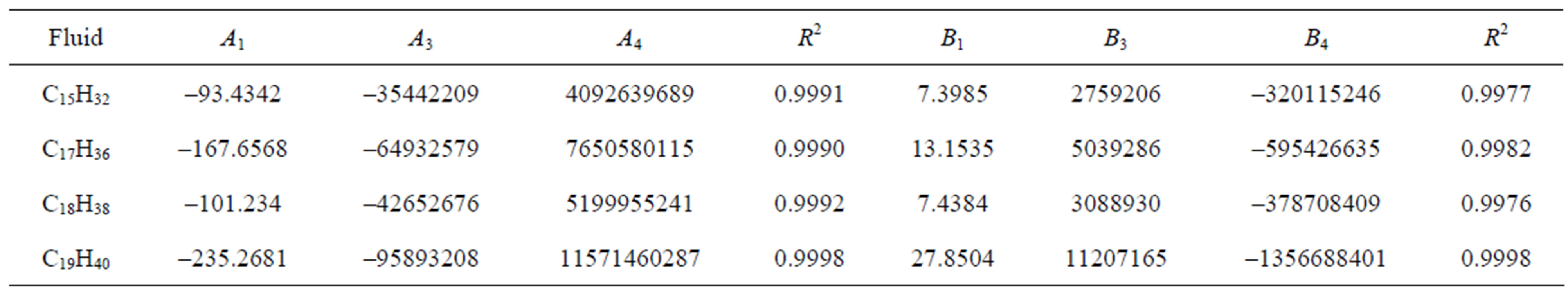
Table 3. The calculated values of A1, A3, A4, using Equation (11) and B1, B3, B4 using Equation (12) for different fluids and the coefficient of determination (R2).

Figure 4. The thermal pressure coefficient values using LIR(0), versus density for C18H38 fluid compared with the thermal pressure coefficient using LIR(1) and LIR(2) at 333.15 K.

Figure 5. The thermal pressure coefficient values using LIR(0),versus density for C18H38 fluid compared with the thermal pressure coefficient using LIR(1) and LIR(2) at 343.15 K.
4. Results
In this paper, we derive an expression for as the thermal pressure coefficient of C15H32, C17H36, C18H38 and C19H40 dense fluids using the linear isotherm regularity[1,3,18]. Unlike previous models, it has been shown in this work that, the thermal pressure coefficient can be obtained

Figure 6. The thermal pressure coefficient values using LIR(0), versus density for C19H40 fluid compared with the thermal pressure coefficient using LIR(1) and LIR(2) at 333.15 K.

Figure 7. The thermal pressure coefficient values using LIR(0),versus density for C19H40 fluid compared with the thermal pressure coefficient using LIR(1) and LIR(2) at 343.15 K.
without employing any reduced Helmholtz energy [9-15]. Only, pVT experimental data have been used for the calculation of the thermal pressure coefficient. Comparison of the calculated values of the thermal pressure coefficient using the linear isotherm regularity with the values obtained experimentally show that validity of the use of the Linear isotherm regularity for studying the thermal pressure coefficient of dense fluids of the monatomic is doubtful [18]. The validity of the use of the linear isotherm regularity equation state for calculating the thermal pressure coefficient of dense fluids of the polyatomic is not also precise [5]. In this work, it has been shown that the temperature dependences of the intercept and slope of using linear isotherm regularity are nonlinear. This problem has led us to try to obtain the expression for the thermal pressure coefficient using the extending the intercept and slope of the linearity parameters versus inversion of temperature to 2 order. The thermal pressure coefficient are predicted from this simple model are in good agreement with experimental data. The results show the accuracy of this method is general quite good.
5. Acknowledgements
The authors thank the Payame Noor University for financial support.
NOTES