1. Introduction
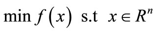
System of convex equations is a class of problems that is conceptually close to both constrained and unconstrained optimization and often arise in the applied areas of mathematics, physics, biology, engineering, geophysics, chemistry, and industry. Consider the following system of convex equations
 (1)
(1)
in which  is a convex continuously differentiable function. It is noticed that if
  the system (1) is a linear system of equations and there are a lot of approaches to solve this problem. One of the most interesting methods for solving linear system is fixed point methods that have been comprehensively studied by many authors. For example, shrinkage, subspace optimization and continuation [1], fixed-Point continuation method [2], nonlinear wavelet image processing [3], EM method [4], iterative thresholding method [5] and fast iterative thresholding [6]. The system (1) is called an overdetermined system whenever
  and under-determined for
 . If
. If , we obtain a square system of convex equations. Most of the time, we wish to find a proper
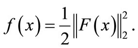
  such that (1) holds as closely as possible. This means that our objective is to reduce
  as much as and, if possible, reduce it to zero. Hence the system of convex Equations (1) can be written as an unconstrained optimization problem
 (2)
(2)
in which
 (3)
(3)
It is obvious that
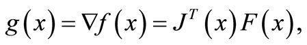
where  is the Jacobin matrix of
 . In this work, we consider a
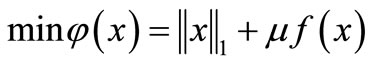
  -regularized least squares problem for system (1):
 (4)
(4)
in which  is a parameter. We note that if
  and any
  is convex, then F is convex. On the other hand, convexity of
  implies that f is convex. Therefore, φ is a convex function.
As an example, Hale, Yin, and Zhang in [2] presented a fixed-point continuation method for  -regularized minimization that based on operator-splitting and con tinuation:
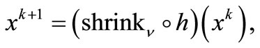 (5)
(5)
in where  and mappings
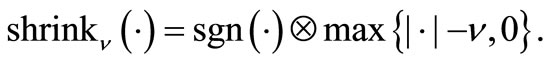
  are defined as :
 (6)
(6)
 (7)
(7)
The operator  in the right hand side of relation (7) denote the component-wise product of
  and
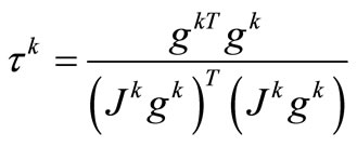
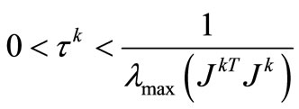
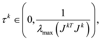
and . Because of the parameter τ is constant, the number of iterations and computational costs increase and so it is not suitable. To overcome the mentioned disadvantage, we create innovation in the parameter τ based on the steepest descent direction:
 (8)
(8)
The analysis of the new approach shows that it inherits both stability of fixed point methods and low computational cost of steepest descent methods. We also investigate the global convergence to first-order stationary points of the proposed method and provide the quadratic convergence rate. To show the efficiency of the proposed method in practice, some numerical results are also reported.
The rest of this paper is organized as follows: In Section 2, we describe the motivation behind the proposed algorithm in the paper together with the algorithm’s structure. In Section 3, we prove that the proposed algorithm is globally convergent. Preliminarily numerical results are reported in Section 4. Finally, some conclusions are expressed in Section 5.
2. The New Algorithm: Motivation and Structure
In this section, we first introduce a fixed point algorithm for small-scale convex systems of equations. Then, given some properties of the algorithm and investigate its global convergence as well as the quadratic convergence rate. The objective function in (4) is a sum of two convex functions. By convex analysis, minimizing a convex function  is equivalent to finding a zero of the subdifferential
 . Let
. Let  be the set of optimal solutions of (4). It is well-known that an optimality condition for (4) is
or equivalently,
 (9)
(9)
where 0 denotes the zero vector in  and
and  is i-th component of
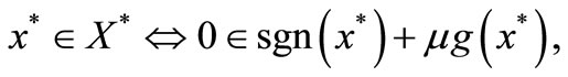
 . It follows readily from (9) that 0 is an optimal solution of (4) if and only if
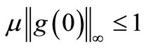 , or in other words,
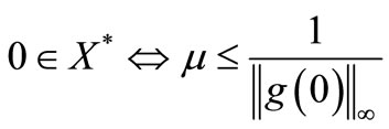
Therefore, it is easy to check whether 0 is a solution of (4) (see [2]).
One of the simplest methods for solving (4) generates a sequence  that based on steepest descent direction. Here,

and . Note that if the system (1) be a linear system of equations, then
  and
and
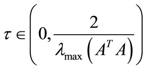 . Here, the system (1) is a convex system of equations, then
 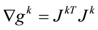 and for the purpose of our analysis, we will always choose
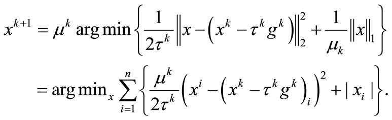
 . Using these information, we present a proximal regularization of the linearized function f at
  for problem (4) (see [7]), and written it equivalently as
 (10)
(10)
After ignoring constant terms, (10) can be rewritten as
 (11)
(11)
Notice that the function in the problem (11) is minimized if and only if each functions
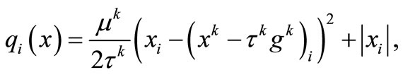
is minimized. If we take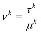 , then we can simply obtain the minimizer of
  as follows:
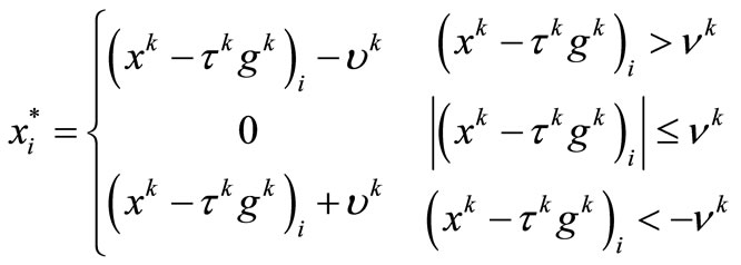
Therefore,  and the solution of (4) is obtained. Now, based on above arguments, a new fixed point algorithm can be outlined as follows:
Algorithm 1: Fixed point algorithm (FP)
Input: Choose an initial point  and constants
 ,
,  ,
, .
.
Begin
 ;
;  l
l
While  {Start loop }
Step 1: {Parameter shrinkage calculation}

Step 2: {Operation shrinkage calculation}
Step 3: {Parameters update}
Calculate  as (8);
Generate ;
;
Increment k by one and go to Step 1;
End While {End loop}
End
3. Convergence Analysis
In this section, we will give the convergence analysis of the proposed algorithm given in Section 2. In the convergence analysis, we need the following assumption:
(H1) Problem (4) has an optimal solution set , and there exists a set

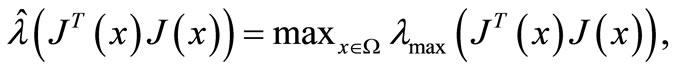
for some  and
and , such that f is twice continuously differentiable on Ω and
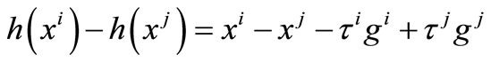
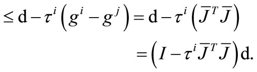
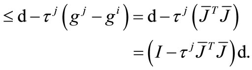
for all . Using the mean-value theorem, we hav
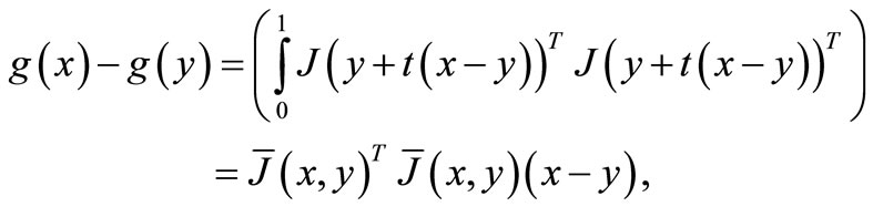
for any .
.
(H2) There exists a constant  such that
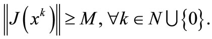
Lemma 3.1. By the definition of  and
and  satisfying (8), we have

for any .
.
Proof. Suppose that  then
then  and
and . So by (8), we conclude that
 . Now suppose that
 . Then, we show that
 . By contradiction, we assume that
 . Then
  and
and .
.
Therefore we have  that is a contradiction.
In the following lemma, we show that the new choice of  satisfying in the lemma 4.1 and corollary 4.1 of [2] when
 .
.
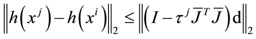
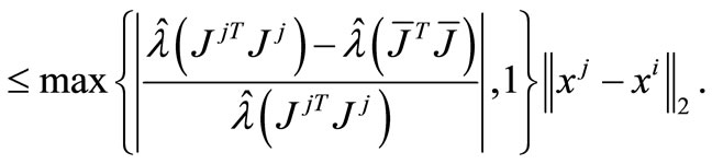
Lemma 3.2. Under assumption (H1), the choice of  and
and  result in
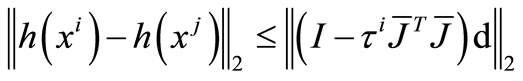
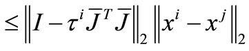
  is nonexpansive over Ω, i.e. for any
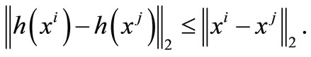 (12)
(12)
Moreover,  whenever equality holds in (12).
Proof. Let  and
and . Now, we have two cases:
1) If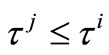 , then
 (13)
(13)
Hence,


Let . By the lemma 3.1, we have
  if and only if
 .
.
Then

if by the equation (13), we obtain
which contradicts to .
.
Hence  so that
2) If , then
 (14)
(14)
Hence,


Let . By the lemma 3.1, we have
 if and only if
 .
.
Then

if by the Equation (14), we obtain

which contradicts to . Hence
so that
which completes the proof.
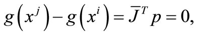
Corollary 3.3. (Constant optimal gradient). From (H1) assumption, for any , there is a vector
  such that
 .
.
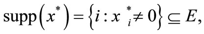
Let  be the solution set of (4),
  , and
, and  be the vector specified in corollary 3.2. Then, we define
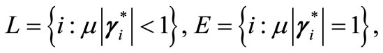
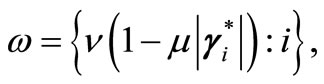
where . We will show that the sequence generated by (5) is finite convergence for components in L and is quadratic convergence for components in E.
It is obvious from the optimality condition (9) that , and for any
 , we have
Hale, Yin, Zhang in [2] establishes the finite convergence properties of  stated in the following of theorem. The proof of the theorem 3.4 and 3.5 is similar to the theorem 4.1 and 4.2 in [2].
Theorem 3.4. Under assumption (H1), the sequence  is generated by the fixed point iteration (5) applied to problem (4) from any starting point
  converges to some
 . In addition, for all but finitely many iterations, we have
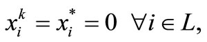 (15)
(15)
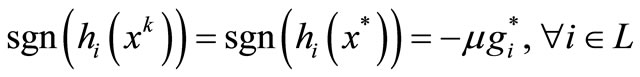 (16)
(16)
where the numbers of iterations not satisfying (15) and (16) do not exceed  and
and , respectively.
Theorem 3.5. (The quadratic case). Let f be a convex quadratic function that is bounded below,  be its Hessian, and
  satisfy
then the sequence  is generated by the fixed point iteration (5) applied to problem (4) from any starting point
  converges to some
 . In addition, for all but finitely many iterations, we have (15) - (16) hold for all but finitely many iterations.
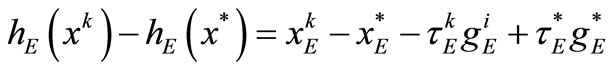
Lemma 3.6. Suppose assumptions (H1) and (H2) holds. Then, we have

Proof. From (9), we can obtain
then, by (H2) and the above inequality, we have
For sufficiently large k, we conclude that
Now, consider the sequence generated by the FP algorithm. According to the fixed point iterations (5), it converge to some point
 . We will show that the convergence is quadratic. In order to do, the following additional assumption is required:
(H3) The following condition
 (17)
(17)
holds, in where 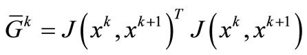 and
and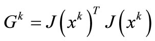 . Suppose that k is enough large so that
 , for all
 . Also, suppose that
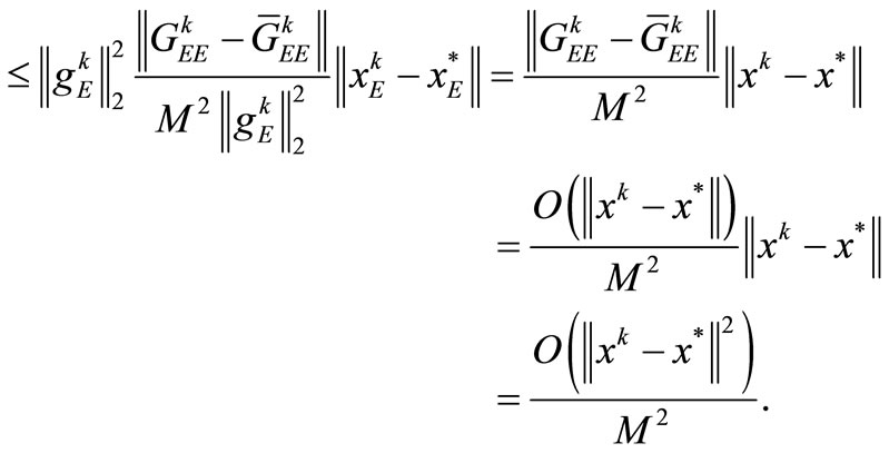
denote the square sub-matrix of the matrix C corresponding to the index set E. Firstly we suppose that , then the mean-value theorem yields
 (18)
(18)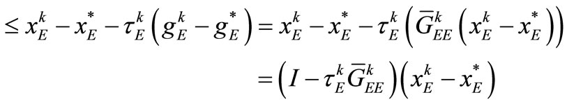
Since 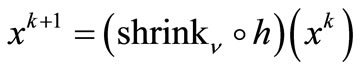 and
and  is non-expansive [2], using H2, (17), and (18), we have that


Secondly, we suppose that . Similar first case, we conclude that
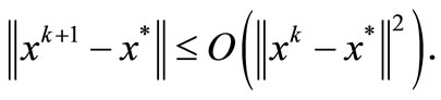
Theorem 3.7. Suppose that (H1)-(H3) holds and let  is the sequence generated by the FP algorithm starting
 . For sufficiently large k, the sequence
  is converges to some point in
  quadratically.
4. Preliminary Numerical Experiments:
This section reports some numerical results and comparisons regarding the implementations of the new proposed idea of the present study with some other algorithms for small-scale problems. All codes are written in MATLAB 9 programming environment with double precision format by a same subroutine. In the experiments, the presented algorithms are stopped whenever

Test problems are as follows:
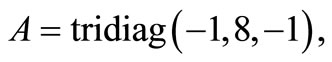
1) Tridiagonal system linear is

in where A is a  tridiagonal matrix given by
and
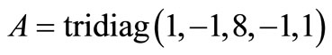
2) Five diagonal system linear is
in where A is a  five matrix given by
and

3) Logarithmic function [8]
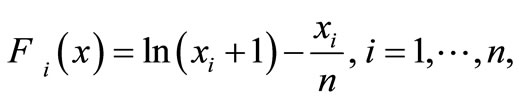
initial point: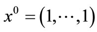 .
.
4) Strictly convex function 1 [8]  that is the gradient of
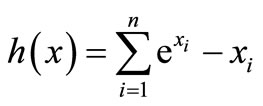
initial point: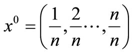 .
.
5) Strictly convex function 2 [8]  that is the gradient of
initial point: .
.
6) Strictly convex function 3 [8]  that is the gradient of
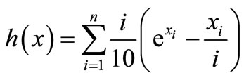
initial point: .
.
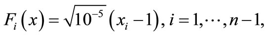
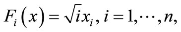
7) Linear function-full rank [8]
initial point: .
.
8) Penalty function [8]

initial point: .
.
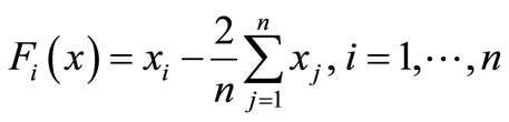
9) Sum square function [9]
initial point: .
.
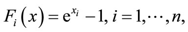
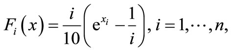
10) Trigonometric exponential function [10]

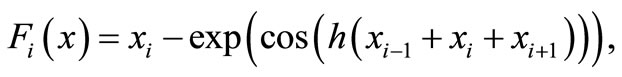
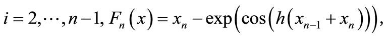
where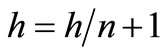 .
.
initial point: .
.
In this section, we compare the numerical results obtained by running Algorithms following:
1) FP1 
2) FP2 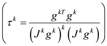
3) DS (steepest descent direction,

in where the Jacobian matrix Jk is exact. In running the algorithm FP1 and FP2 takes advantages of the parame - ters
 and
and . The dimensions of problems are selected from 2 to 100. The results for small-scale problems are summarized in Table 1.
In Table 1,  and
and  respectively indicate the total number of iterates and the total number of function evaluations. Table 1 indicates the total number of iterations and function evaluations for some small scale problems with dimensions 2 to 100. Evidentally, one can see that FP2 performs better than the other presented algorithms in the sense of both the total number of iterations and the total number of function evaluations. From Table 1, we observe that the proposed algorithm is the best one on the all of test problems. We can deduce that our new algorithm is more efficient and robust than the other considered algorithms for solving small scale system of convex equations problems. In more details, the results of Table 1 in Figure 1 are interpreted thanks to the Dolan and More’s performance profile in [11].
In the procedure of Dolan and More, the profile of each code is measured considering the ratio of its computational outcome versus the best numerical outcome of all codes. This profile offers a tool for comparing the performance of iterative processes in statistical structure. In particular, let S is set of all algorithms and P is a set of
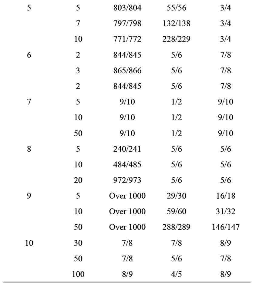
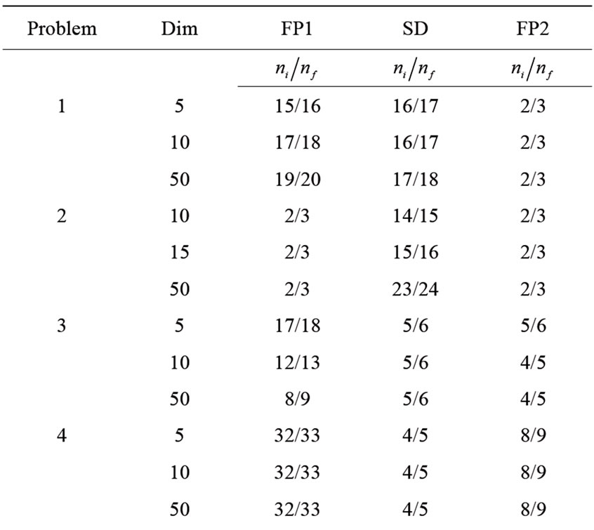
Table 1. Numerical results for small scale problems.
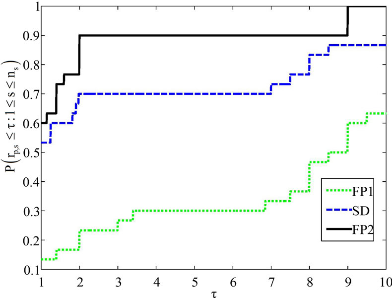
Figure 1. Performance profile for the number of iterates.
test problems, with  solvers and
  problems. For each problem p and solver s and
  is the computation result regarding to the performance index. Then, the following performance ratio is defined
 (19)
(19)
If algorithm is not convergent for a problem p, the procedure sets
 , where
  should be strictly larger than any performance ratio (19). For any factor
 , the overall performance of algorithm
 is given by
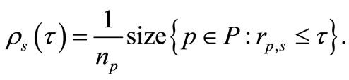
In fact  is the probability of algorithm
  that a performance ratio
  is within a factor
  of the best possible ratio. The function
  is the distribution function for the performance ratio. Especially,
  gives the probability that algorithm s wins over all other algorithms, and
  gives the probability of that algorithm s solve a problem. Therefore, this performance profile can be considered as a measure of the efficiency and the robustness among the algorithms. In Figure 1, the x-axis shows the number
  while the y-axis inhibits
From Figure 1, it is clear that FP2 had the most wins compared with the other algorithm while it solved about 60% of the test problems with the greatest efficiency. If one concentrates on the ability of completing a run successfully, it can be seen that FP2 is the best algorithm among the considered algorithms because it reaches faster than the other.
5. Conclusion
In this paper, we have presented a new algorithm for small-scale systems of convex equations that blending steepest descent direction and fixed point ideas. Preliminary numerical effort on the set of small-scale convex systems of equations indicates that significant profits in both the total number of iterations and the total number of function evaluations can be achieved.