Telegraph Equations and Complementary Dirac Equation from Brownian Movement ()
1. Introduction
The relativistic propagator for a free particle in  space can be obtained [1-5] from the considerations of the statistics of random walks in space and time without restoring to formal analytic continuation. It has been shown [6] that the wave functions and propagators that occur in classical equations are themselves observables on the lattice in contrast to quantum mechanics where wave functions are rather mysterious objects which only facilitate calculations and which are not themselves observables. It has also been shown [7] that the free particle classical Schrödinger’s equation in
  space occurs naturally in the description of correlations in random walks on the lattice where the wave-function solutions describe the features of ensembles of random walks. In recent attempt a stochastic model of the telegraph equation due to Kac [8] and Gaveau et al. [9] has been extended [10] to obtain Dirac Equation for a particle in electromagnetic field using Brownian motion in time as well as space. Recently, the relativistic diffusion processes have been discussed in random walk models [11] and the quantization of Brownian motion have been worked out [12].
In our earlier papers [13-15] the diffusion equation and classical Schrödinger’s equation for free particle and also for a particle under a force field have been derived as complementary equations from the Brownian motion and it has been shown that the continuum limit which transforms this classical Schrödinger’s equation into the usual Schrödinger’s quantum equation without using any formal analytic continuation and the wave-particle duality, is simply Heisenberg’s uncertainty relation between position and momentum of the Brownian particle. Extending this work in the present paper by putting a finite speed cutoff into the diffusion process we have obtained telegraphic equations to describe particle densities in Brownian movement on a lattice site and showed that the complementary classical Dirac equation appears naturally as the consequence of correlations in particle trajectories in Brownian movement. Here the constituents of wave-function describe the features of ensembles of random walks on lattice and hence the observables are easily interpreted. We have also derived the condition which transforms this classical Dirac equation for Brownian movement into usual Dirac’s relativistic quantum equation and it has been demonstrated that this condition is basically Heisenberg’s uncertainty relation for energy and time.
2. Telegraphic Equations from Brownian Movement
Let us work in 2-dimensional spatial-temporal space  on a lattice with spatial and temporal spacings d and e respectively and assume
  as the probability that a particle arrives in the state
  at x, t where these four states have been assigned to the particles to keep the track of correlation in the trajectories as they move between lattice sites such that the state- 1 and state-3 correspond to the particle moving to the right and state-2 and state-4 correspond to the left moving particles. The state-1 and state-3 are separated by an odd number of transitions from right moving to the left moving and similarly, state-2 and state-4 are separated by an odd number of left to right transitions. At each lattice site, the Brownian particles choose whether to go left or right at the next step. Let us assume that the particles maintain the same direction with probability p and change the direction with probability q such that
 (2.1)
(2.1)
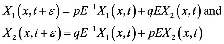
Then we write the difference equations for the ensemble of particles as
 (2.2)
(2.2)
which is the master set of equations for the ensemble of random walks giving the distribution of particles in the four states.
Let us have
 (2.3)
(2.3)
which is proportional to the probability that a particle arrives at  in any state.
Let us also define
 (2.4)
(2.4)
which gives the direction difference. If the number of left moving and right moving particles are the same in the beginning then we have
 (2.5)
(2.5)
Let E be the shift operator with respect to x coordinate. i.e.,
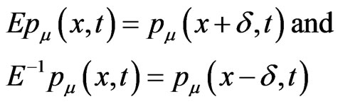 (2.6)
(2.6)
Then using Equations (2.1) to (2.6), we get
 (2.7)
(2.7)
If we choose

then Equation (2.7) reduce to
 (2.8)
(2.8)
Expanding shift operator in terms of differential operator , we get
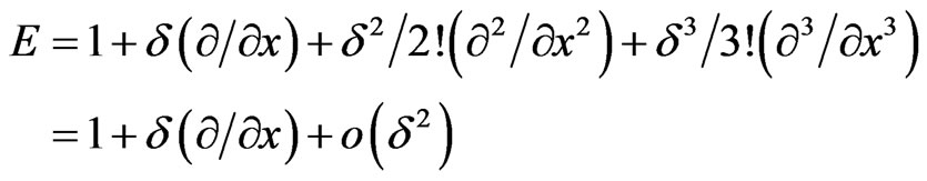
Ignoring the term of order higher than d, it gives
 (2.9)
(2.9)
where n is any integer. Then Equation (2.7) reduce to
 (2.10)
If each particle persists at constant speed c along its current direction for an average time  then
then
 (2.11)
and
 (2.11a)
which gives
 (2.11b)
These equations show that each particle changes its direction with the average frequency μ and persists at constant speed c between two consecutive changes of directions. For such a periodic motion the mean free path
 (2.12)
plays the role of the wave length.
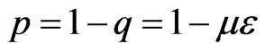
Substituting the limits (2.11) and values of p and q from Equations (2.11a) and (2.11b) into Equation (2.10), we get
 (2.13)
Then Equations (2.8) reduce to the following form
 (2.14)
where 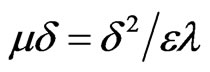 and it may be ignored if we retain the terms of only first order in d and then Equations (2.13) and (2.14) respectively reduce to the following forms:
 (2.15)
 (2.16)
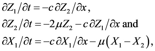
where Equations (2.16) give a particular form of Telegraph equations.
Imposing the condition (2.5), Equations (2.15) are further reduced to
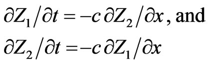 (2.17)
which give another form of Telegraph equations.
3. Classical Dirac Equation
Let us denote the expected excess in the number of Brownian particles moving in a given direction by parity,
 (3.1)
(3.1)
which correspond to the expected difference in the number of even and odd parity paths to a given point. Then using Equation (2.2) we have
 (3.2)
(3.2)
The ensemble of particles, described by master Equations (2.2), change its state with each step and it takes eight time steps for the ensemble to return to its initial statistical state in the sense that the expected number of direction changes per particle is four [6]. Thus the Equation (3.2) in the continuum limit is iterated for eight time steps i.e.
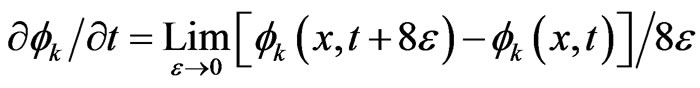 (3.3)
(3.3)
where k = 1, 2, and
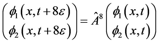 (3.4)
(3.4)
with

or
 (3.5)
(3.5)
under the approximation (2.9). Here under the first order approximation various powers of p, given by (2.11b) may be written as

and then Equation (3.5) becomes
 (3.6)
(3.6)
Substituting this result into Equation (3.4) and using Equation (3.3), we get
 (3.7)
(3.7)
Let us write
 (3.8)
(3.8)
Then Equation (3.7) become
 (3.9)
(3.9)
Let us revert the Brownian motion such that the statesone and three correspond to particles moving to the left while the states-two and four correspond to right moving particles. In this case the states-one and three will be separated by an odd number of transitions from left moving to right moving and the states-two and four will be separated by an odd number of right to left transitions. Then the master Equations (2.2) will be transformed to
 (3.10)
If 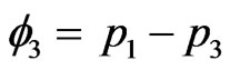 and
and  are the expected excesses in the number of left moving and right moving particles respectively, then we have
 (3.11)
Then Equation (3.4) becomes
 (3.12)
where
 (3.13)
Thus in place of Equations (3.7), we have
 (3.14)
Let us choose

Then Equation (3.14) reduce to
 (3.15)
If we define the function
 (3.15a)
then Equations (3.9) and (3.15) may be written as
 (3.16)
where 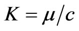 and g1 and g4 are 4 × 4 matrices defined as
 (3.17)
satisfying the conditions
 (3.18)
These equations may be generalized in to the following form in three dimensional spatial coordinates;
 (3.19)
where m = 1, 2, 3, 4 with  and g2 and g3 are given by
 (3.20)
which satisfy the following conditions
 (3.18a)
These matrices also satisfy the following conditions with matrices g1 and g4 given by Equation (3.17);
 (3.18b)
The conditions (3.18), (3.18a) and (3.18b) may be combined into following form
 (3.21)
These matrices constitute Majorana representation of Dirac operators and hence Equation (3.19) may be called classical Dirac equation which becomes usual relativistic Dirac equation for
 ,(3.22)
where c is the velocity of light and  with h as Planck’s constant
This condition may be interpreted as

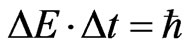
But we have already seen that  where ∆t is the average time for which each particle in the Brownian motion persists at constant speed c along its current direction. moc2 is its rest energy during ∆t and thereafter it changes the direction. In other words in the time interval ∆t the change of energy is ∆E = moc2. Then the condition (3.22), under which the classical Dirac equation becomes the Dirac’s relativistic quantum equation, is
 (3.23)
which is Heisenberg’s uncertainty relation for energy and time.
4. Discussion
Equations (2.16) and (2.17), obtained from the Brownian movement represented by master Equations (2.2), give two different forms of Telegraph equation. The classical Dirac Equation (3.16) in one spatial dimension and its generalization into the form given by Equation (3.19) appear naturally as the consequence of master Equations (2.2) and (3.10) of Brownian movement, where the constituents of y, given by Equation (3.15a), have the meaning on the lattice and denote the limits of ensemble averages of excess parities. These functions are not just the calculational tools and the function y describes the features of ensembles of random walks on lattice and hence the observables are easily interpreted in contrast to the usual quantum mechanics.
The conditions (3.22) which transforms the classical Dirac equation for Brownian movement into usual Dirac’s relativistic quantum equation, is basically Heisenberg’s uncertainly relation (3.23) for energy and time. The usual formal analytic continuation which is necessary to relate the classical and quantum equation is completely absent here and hence the interpretation of quantum mechanics here is direct one without the problems of measurements usually associated with quantum mechanics. Here the derivation of Dirac equation is a sensible classical scheme to produce many particle simulations of quantum mechanics where quantum equation exists as a description of classical theory (Brownian movement).
In our earlier papers [13-15] it has been shown that for transforming the classical Schrödinger’s equations, obtained as the consequence of Brownian movement, into usual Schrödinger’s quantum equation the necessary condition is Heisenberg’s uncertainty relation between position and momentum of the Brownian particle. In the light of this result and the forgoing discussion it may be concluded that the classical equations for ensemble averages of excess parity in Brownian movement can be transformed into usual Schrödinger’s equation by imposing Heisenberg’s uncertainty relation between position and momentum of Brownian particle and the similar classical equations can be transformed into usual Dirac’s equation by imposing the uncertainty relation between energy and time associated with Brownian particle without using a formal analytic continuation and wave-particle quality. These results support the recent work [16] on the role of generalized uncertainty principle in the development of quantum mechanics from classical context. These results partially support the earlier work [1-5] showing that the quantum mechanical equations are the derived properties of the binomial distribution and no formal analytic continuation is required to produce them. Some results of this paper shall be helpful in framing the foundation of space-time path formalism [17] for relativistic quantum mechanics. We shall undertake the study of this problem in our forthcoming paper.
NOTES