A Recursive Binary Tree Model for the Analysis of the Response to Antiretroviral Therapy of HIV Infected Adults in Burkina Faso

Simon Tiendrébéogo^1,2, Séni Kouanda², Blaise Somé¹, Simplice Dossou-Gbeté³

¹Laboratoire d’Analyse Numérique, d’Informatique et de BIOmathématiques, Université Ouaga I Pr Joseph KI ZERBO, Ouagadougou, Burkina Faso.
²Département Biomédical et Santé Publique, Institut de Recherche en Sciences de la Santé, Ouagadougou, Burkina Faso.
³Université de Pau et des Pays de l’Adour, E2S UPPA, CNRS, LMAP, Pau, France.

DOI: 10.4236/ojs.2019.96041                

Abstract

In this paper we aim to analyse temporal variation of CD4 cell counts for HIV-infected individuals under antiretroviral therapy by using statistical methods. This is achieved by resorting to recursive binary regression tree approach [1] [2]. This approach has made it possible to highlight the existence of several segments of the population of interest described by the interactions between the predictive covariates of the response to the treatment regimen.

Keywords

Model-Based Conditional Regression Tree, CD4 Cell Count Prediction, Linear Mixed Model, Stability Analysis, Antiretroviral Therapy

1. Introduction

SubSaharan Africa’s population is among the most HIV infected in the world. In 2014, there were 1.4 million (1.2 - 1.5 million) new infections and around 790,000 (690,000 - 990,000) people died of AIDS-related illnesses [3]. These alarming statistics indicate a generalised HIV epidemic. On the one hand, HIV/AIDS infection is correlated with high risk behaviors such as occasional unprotected sex. On the other hand, the burden of the disease is correlated with poverty, weakness of health system, discrimination toward girls and women, low education level, malnutrition, migration, stigmatization of persons living with HIV/AIDS (PLWHA) and low volume of funding for the fight against HIV/AIDS [4] [5]. In addition, PLWHA are sometimes less observant during the treatment period or co-infected by Tuberculosis and then may face failure of treatment [6] [7].

In Burkina Faso, the overall HIV prevalence was estimated to be 1.8% in 2003 [8]. The antiretroviral therapy (ART) program started in 1999 with the financial support of international funding institutions and NGOs [9]. The Global Fund to Fight against AIDS, Malaria and Tuberculosis was the leading funding program between 2003 and 2007 [10]. Its intervention in Burkina Faso was the subject of an evaluation at the end of the five-year period 2003-2007. It aimed at measuring the intervention effects on health service access as well as HIV/AIDS related morbidity and mortality. Among other questions that deserve additional attention, there is that of the effectiveness of care through the analysis of the response to treatment of people who benefited from it. Viral load and CD4 cells count are relevant indicators that can be considered for such an investigation. CD4 cells count is low cost, simple to measure and a good predictor of the HIV dynamics during treatment [11]. Since it is unclear how health conditions at the beginning of treatment and the demographic characteristics are correlated to the temporal variations of CD4 cells count, we propose to address this gap in this paper. The aim of this study is to model temporal variations of CD4 cell counts in a sample of ART patients with a longitudinal tree regression approach.

2. Data

Data come from the Global fund to fight AIDS, Tuberculosis and Malaria Five year evaluation survey database. The sample included both male and female older than 15 that had initiated ART between 1st Jan 2003 and 31st Dec 2007. Data consisted of socio-demographic characteristics and semesterly CD4 count evaluations during the follow-up period. More details on patient sampling and data collection can be found in [6]. Finally, we applied the following patient selection criteria: at least two CD4 counts available of which one is the baseline CD4 count; first line ART regimen, and baseline WHO clinical stage available.

We also applied two operations to complete cases. First, we created 3 new variables: body mass index (BMI) and the CD4 count evaluation clinical visit index (Time). Then we corrected the positive asymmetry of the distribution of CD4 count by applying a square root transformation.

Baseline Data Description

Our study included 3459 ART patients from 14 ART centres. Most centres (98%) were urban. For most patients (95%), the regimen consisted of two nucleoside reverse transcriptase inhibitors (NRTI) plus one non-nucleoside reverse transcriptase inhibitor (NNRTI). Table 1 shows that 72% were female, 70% were married, 95% were infected by HIV1, 81% initiated ART at WHO clinical stages between 3 and 4, and 83% had CD4 count lower than 200. The median age at ART initiation was 35 (30; 40).

Table 1. Patients’ characteristics.

Note: 1) NGO: non-governmental organization; CDT: Centre de Dépistage et de traitement de la Tuberculose; CTA: Centre de Traitement Ambulatoire; CDVA: Centre de Dépistage Volontaire et Anonyme. 2) We used Kruskall-Wallis and Mann-Whitney tests to compareCD4counts distribution.

3. Statistical Methodology

3.1. Statistical Model

The statistical model considered in this study for the data analysis belongs to the class of the varying-coefficients regression models as introduced by [12] after [13]. In this setting the regression coefficients are allowed to vary with respect to some covariates called effect modifiers or moderators. When dealing with the framework of the linear model, the dependence of the regression coefficients ${\beta }_j$ of a predictor $X_j$ on effects modifiers should be understood as the expression of an interaction between X and the effects modifiers. Let’s consider a response variable Y conjointly with covariates (X, Z) where $X=\left(X_1,\cdots ,X_p\right)$ and $Z=\left(Z_1,\cdots ,Z_q\right)$. Let’s denote $\mathcal{D}\left(\mathcal{X}\right)$ and $\mathcal{D}\left(\mathcal{Z}\right)$ respectively the spaces of the potential values of X and Z and $\mu \left(x,z\right)=E\left(Y|X=x,Z=z\right)$ with x in $\mathcal{D}\left(\mathcal{X}\right)$ and z in $\mathcal{D}\left(\mathcal{Z}\right)$; the varying-coefficients model will take the following form: $\mu \left(x,z\right)={\beta }_1\left(z\right)x_1+\cdots +{\beta }_p\left(z\right)x_p$. For the present study the functions ${\beta }_j\left(z\right)$ are modeled through a binary tree as follows:

${\beta }_j\left(z\right)={\beta }_{j1}Ind\left(z\in N_1\right)+\cdots +{\beta }_{jK}Ind\left(z\in N_K\right)$

where $\left(N_k,k=1,\cdots ,K\right)$ is rectangular partition of $\mathcal{D}\left(\mathcal{Z}\right)$ and $Ind(\cdot )$ is the indicator function. This choice offers is a flexible way to consider interactions between the covariates Z and the covariates X without a tight specification of such interactions at the model statement step. Moreover this framework allows the identification of subgroups of individuals with specific shape of CD4 variation over time. Finally the model that will be considered for the data analysis will be expressed as follows:

$Y|X=x\mathrm{,}Z=z\mathrm{,}b\sim N\left(x^t\beta \left(z\right)+bI\mathrm{,}{\sigma }^{2}I\right)$ (1)

where

$\beta \left(z\right)={\displaystyle \underset{k=1}{\overset{K}{\sum }}}Ind\left(z\in N_k\right){\beta }_k$ (2)

$b\sim N\left(\mathrm{0,}{\sigma }_b^2\right)$ (3)

and $Ind(\cdot )$ is the indicator function. This is a special case of varying-coefficient regression model [12].

3.2. Model Fitting Methods

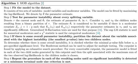
We chose a generalized linear mixed model (GLMM) conditional inference tree algorithm for tree construction [14]. It helps to overcome some instance instability and bias problems that are common in recursive binary tree models fitting [1] [15]. In brief, at each iteration, the algorithm combines the fixed-effect estimation by a model-based partitioning algorithm (MOB) [2] with a linear mixed model random effect prediction. MOB is based on parameter instability tests [16]. Instability refers to a significant difference in coefficient estimates for two subsets of the dataset. The algorithm builds the tree after repetitions of the following steps:

GLMM tree algorithm stopping criterion is based on the linear mixed model log-likelihood denoted $l\left(b\right)$. One strategy to fit the model to data is outlined in the following algorithm [14]:

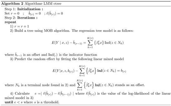
We used R package glmertree [14] for model fitting.

We have looked for an optimal joint value of a minimal terminal node size (minsize) and a numeric significance level $\alpha$ by using Bayesian Information Criterion (BIC). That model selection strategy avoids to choose arbitrary values for minsize and $\alpha$. In our application, the linear mixed model includes two fixed-effects (Treatment and clinical visit index) and one random effect (patient ID). The covariates used to defined the subgroups are Age, Gender, Marital status, baseline CD4 count, WHO clinical stage, the mode of entry into the active list, the history of opportunistic infection at ART initiation, the HIV type and Body Mass Index.

3.3. Stability Analysis and Model Diagnostics

Stability is an essential property of a fitted regression tree model. It ensures that the potential instability of the model is minimized and then the model use, as for prediction task. A model stability can be assessed by fitting the model on data obtained by bootstrap resampling of the training dataset. Variables and cutpoints that were not selected by the original tree may be selected by replicate samples. Metrics for stability assessment include the relative variable selection frequency, the mean frequency of the variable selections per tree and the frequency of each cutpoint over the trees [17]:

• The relative variable selection frequency for a partitioning covariate $z_m$, $m=1,\cdots ,q$ equals the total number of replicate trees that have selected $z_m$ at least once, divided by the total number of replicate trees.

• The mean frequency of the covariate selections per tree for $z_m$ is the total number of times $z_m$ is selected for partitioning by a replicate tree over the repetitions, divided by the total number of replicate trees.

• The relative frequency of a cutpoint $c\left(z_m\right)$ equals the total number of replicate trees that have selected $c\left(z_m\right)$ to split the variable $z_m$, divided by the total number of replicate trees.

A covariate selection is stable if its average split count is close to its number of selections in the original tree and its frequency of selection is close to 100%. Graphical methods are used to analyze variable cutpoints’ variability. A histogram is used to illustrate the cutpoint variability when the partitioning variable is numerical. It is expected that the cutpoints selected in the original tree have the highest frequencies (one or more peaks in the histogram). For an ordered categorical variable, a barplot is used to show the frequency of all possible split points. For an unordered categorical variable, a specific plot is used to visualize the partitions’ variability over the replicates. The same color is used for categories that belong to the same node. The combination of categories that corresponds to a partition observed in the original tree is marked on the right side of the plot by a solid red line. In addition, two dashed lines enclose the area representing the partition. Number(s) on the right side of the area indicate the level(s) of the corresponding split(s) in the original tree. In conclusion, a split point is stable if it is selected by most replicate trees.

We have implemented a non parametric bootstrap method for generalized linear mixed models [18] [19]. Mainly, the method consists of three steps. First, for all $i=1:n$, we computed scalars $b_i^{\mathrm{<mo>\; *\; </mo>}}$ and ${ϵ}_i^{\mathrm{<mo>\; *\; </mo>}}$ by centering and scaling the predicted random variable ${\hat{b}}_i$ and the predicted random variable ${\widehat{ϵ}}_i$ respectively. Consider $\bar{b}$ and $\bar{e}$ the empirical means of $b_i$ and $e_i$. Denote

${\sigma }_b^{*2}=\frac{1}{n}{\displaystyle \underset{i=1}{\overset{n}{\sum }}}{\left({\hat{b}}_i-\bar{b}\right)}^2\text{and}{\sigma }_{ϵ}^{*2}=\frac{1}{n}{\displaystyle \underset{i=1}{\overset{n}{\sum }}}{\left({\hat{e}}_i-\bar{e}\right)}^2$ (4)

the empirical variances of ${\hat{b}}_i$ and of ${\hat{e}}_i$ respectively. The marginal residuals ${\hat{e}}_i$ is also centered and scaled. we compute the predicted values $y^{\mathrm{<mo>\; *\; </mo>}}$ by replacing ${\hat{b}}_i$ by ${\sigma }_b^{\mathrm{<mo>\; *\; </mo>}}{b}^{\mathrm{<mo>\; *\; </mo>}}$ and ${\widehat{ϵ}}_i$ by ${\sigma }_{ϵ}^{\mathrm{<mo>\; *\; </mo>}}{ϵ}^{\mathrm{<mo>\; *\; </mo>}}$. Note that the two random variables follow a standard normal distribution. Thirdly, to obtain each bootstrap dataset, the response y is replaced by a bootstrap of the predicted response $y^{\mathrm{<mo>\; *\; </mo>}}$.

To study the plausibility of the model assumptions, we proceed in two steps. First, we computed the least confounded residuals [20] and assessed the normality assumption using quantile-quantile plot. Secondly, we evaluated the homoscedasticity assumption by plotting predicted values against standardized conditional residuals. For this purpose, we wrote a R code for parametric bootstrap that account for fitted mixed model as add-on for the package stable learner [17] to realize the stability analysis of linear mixed model based recursive binary tree.

4. Results

4.1. Identified Difference in Temporal Variation of CD4 Cell Counts with Respect to Interactions between Covariates

Our model highlights seven subgroups of patients with different temporal variations of CD4 counts (Figure 1). The set of patients at an advanced disease stage (CD4 < 225) is the most splitted. It consists of at least four subgroups of chronological increase of CD4 count. Baseline CD4 count is selected for the first split. It is the most correlated with the temporal variation of CD4 count. Baseline CD4 count is a predictor of sustained virologic response [21]. In the subgroup of patients with baseline CD4 count ≤ 73 cells/μl, Gender is the most correlated with the CD4 count variation. Female patients have a faster chronological increase of CD4 counts than male patients ( ${\hat{\beta }}_2=1.02$ and ${\hat{\beta }}_2=0.82$ respectively).

Figure 1. Conditional inference tree grown on the study dataset. CD4 count is the study outcome. Baseline CD4 count (in CD4), Gender (Genre) and Age were selected as splitting variables. P-value in each edge refers to the smallest p-value found in parameter instability tests.

Uptake and adherence to HIV services may explain this difference. In the subgroup of patient with baseline CD4 counts between 73 cells/μl and 129 cells/μl as well as in the subgroup of patients with baseline CD4 counts between 129 cells/μl and 225 cells/μl, Age is correlated with CD4 count temporal variation. In these subgroups, patients with aged 34 years or below have a slightly higher chronological CD4 count increase compared with older patients. The variable Age selection might be explained by what is called discordant immunological response, likely to happen among older patients [22]. Conversely, the group of patients with baseline CD4 count ≥ 225 cells/μl is homogeneous according to partioning rules.

Table 2 shows a chronological increase of CD4 count on average in all subroups ( ${\beta }_2>0$ and $p\text{-value}<0.05$ ). This finding corroborates the fact that ART treatment aims to reduce the viral load and progressively to restore the immune system. The increase is faster for patients with an initially weakened immune system. On average the ${\beta }_2$ coefficient is small when baseline CD4 count is large. In addition, the ratio ${\hat{\sigma }}_b^2/\left({\hat{\sigma }}^2+{\hat{\sigma }}_b^2\right)=57.07\%$. This shows that individual random effect is important in the analysis of CD4 cell counts time variation.

Subgroups also differ by the difference in treatment response between patients treated with 2NRTI + 1NNRTI regimen and those treated with other ART regimens (2 NRTI + IDV, 2 NRTI + LPV/r, 2 NRTI + NFV). It is commonly admitted that there is no optimal treatment for all patients. Chronological CD4 count levels are higher for patients treated with 2NRTI + 1NNRTI than for those treated with other ART regimens group in the subgroup of patients with baseline CD4 count ≤ 129 and aged 34 and over as well as in the subgroups of patients with baseline CD4 counts between 129 cells/μl and 225 cells/μl (Figure 2). The difference in chronological CD4 count levels between ART regimens is highest

Table 2. Summary of fixed-effects estimation.

Figure 2. Chronological increase of CD4 count in the subgroups identified by the model. Time is in 6-months time scale. (a)-(g) Time (semester).

in patients aged 34 or younger and with baseline CD4 counts between 129 cells/μl and 225 cells/μl. In the remaining subgroups, we found no significant difference ( $p>0.05$ ).

4.2. Conditional Inference Tree Stability Assessment and Model Validation

We performed the stability analysis with 500 bootstrap samples. Relative frequencies of selecting baseline CD4 count, Gender, Age are all equal to 100% (Table 3 and Figure 3). Their mean frequency of selections per tree are respectively equal to their selection frequency in the initial tree (Table 3). In addition, Figure 4 shows that all the bootstrap trees have splitted baseline CD4 count on the same levels as in the initial tree. Age is splitted at age 34 on level 3 as in the original tree. Similarly, Gender is splitted on level 3. Thus, baseline CD4 count, Gender and Age can be considered as stable. Most of the bootstrap trees (97.6%) and the original tree are identical (Figure 3). Finally, variable EntryMod need not be retained. It is only selected by 2.4% of bootstrap trees. To sum up, the fitted tree is stable. Finally, Figure 5 and Figure 6 show that there is no evidence against normality and homoscedasticity assumptions respectively.

Figure 3. Frequencies of the different trees built over the repetitions. Dashed horizontal red lines mark the frequency of the original tree. It is enclosed by a solid vertical red line at the right of the plot.

Figure 4. Stability of the cutpoints selection for partioning. Dashed vertical lines mark the original tree cutpoints. The number above a dashed vertical red line indicates the level at which the split occurred in the tree. For example, Age is splitted twice on level 3. For the categorical variable Gender, the split occurred between Male and Female on the level 3 in the original tree.

Figure 5. Quantile-quantile plot of standardized least confounded residuals.

Figure 6. Homoscedasticity assumption evaluation plot.

Table 3. Variable selection overview.

5. Discussion and Concluding Remarks

In this study, we have analyzed data from a retrospective cohort of adults who started Antiretroviral Therapy at different centres between 2003 and 2007 in Burkina Faso. The results showed that the population of ART patients in Burkina Faso may be split into seven subgroups, according to the CD4 count variation over time. The number of the subgroups indicates that this population is heterogeneous as regards treatment response. This feature is particularly pronounced among advanced infected patients (CD4 < 225). The high proportion of patients (83%) in this condition may partly explain this finding. Gezie et al. [24] found Age as a predictor of CD4 counts over time in Ethiopia. Younger age was positively correlated to CD4 count increase during the course of treatment. But no cutpoint was provided to allow a comparison with our finding.

On average, we have observed an increase of CD4 counts in all subgroups. This finding confirms the benefit of ART treatment whatever the patients’ health conditions. However, CD4 counts do not recover a normal value when ART is started at a low baseline CD4 count [25] [26]. In addition, we found that the increase is lower among patients with greater baseline CD4 counts. Garcia et al. reported that the lower increase was not observed when it was adjusted by viral load at last determination [21]. This study reveals that female patients have a faster increase than male patients. This can be explained by representations of masculinity in Burkina Faso that could lead to late presentation and poor compliance with treatment [27] [28].

Another finding of this study is that there are differences in treatment response between patients treated with 2 NRTI + 1 NNRTI regimen and those treated with other ART regimens (2 NRTI + IDV, 2 NRTI + LPV/r, 2 NRTI + NFV) in the groups of patients with baseline CD4 between 73 and 225. The differences could be related to a better adherence to ART regimen in the subgroups. Protease inhibitors are expected to be more effective than 1 NNRTI. But tolerance to treatment may explain why they are less effective.

Abrogoua et al. [29] have also shown a heterogeneity in the population of patients under ART in Cote d’Ivoire. Their study identified four and fourteen CD4 counts variation subgroups in two samples of ARV-treated patients enrolled in a clinical trial between 2006 and 2007 and followed for two years in Cote d’Ivoire. The samples included 87 nevirapine treated patients and 164 efavirenz treated patients respectively. Age, sex, weight, Karnofsky’s score, haemoglobin, occurrence of an opportunistic infection were used for CD4 cell counts modeling. Unlike Abrogoua et al. [29], we studied 3459 HIV infected patients followed up to five years in routine clinical practice. In addition, we included the treatment regimen in the model.

Acknowledgements

A part of this work was carried out during a stay of the first author as a doctoral student at the Laboratoire de Mathématiques et de leurs Applications de Pau (LMAP), at the Université de Pau et des Pays de l’Adour (UPPA). He is grateful for the welcome given to him by the members of LMAP and for having benefited from its resources. Authors thank Dr. Stephen Centrella and Mrs Marie Henriette Somda for their kind assistance in the English writing.

Author Contributions

Simon Tiendrébéogo: Analyzed data, wrote analysis tools and wrote the paper.

Séni Kouanda: Contributed to write the paper and provide guidance on the clinical interpretation of the findings.

Blaise Somé: Contributed to write the paper and reviewed the manuscript.

Simplice Dossou-gbété: Contributed to the data analysis and to the writing of both analysis tools and the paper.

Ethics

This article is original and contains unpublished material. The corresponding author confirms that the other authors have read and approved the manuscript and no ethical issues involved.

Conflicts of Interest

The authors declare no conflicts of interest.

References

[1]	Hornik, K., Hothorn, T. and Zeileis, A. (2006) Unbiased Recursive Partitioning: A Conditional Inference Framework. Journal of Computational and Graphical Statistics, 15, 651-674. https://doi.org/10.1198/106186006X133933
[2]	Zeileis, A., Hornik, K. and Wien, W. (2008) Model-Based Recursive Partitioning Torsten Hothorn. Journal of Computational and Graphical Statistics, 17, 492-514. https://doi.org/10.1198/106186008X319331
[3]	WHO (2015) Global Health Sector Response to HIV, 2000-2015 Focus on Innovations in Africa. Technical Report.
[4]	Muula, A.S., et al. (2007) Gender Distribution of Adult Patients on Highly Active Antiretroviral Therapy (HAART) in Southern Africa: A Systematic Review. BMC Public Health, 7, Article No. 63. https://doi.org/10.1186/1471-2458-7-63
[5]	Schoepf, B.G. (2010) Assessing AIDS Research in Africa: Twenty-Five Years Later. African Studies Review, 53, 105-142. https://doi.org/10.1353/arw.0.0252
[6]	Kouanda, S., et al. (2011) Determinants and Causes of Mortality in HIV-Infected Patients Receiving Antiretroviral Therapy in Burkina Faso: A Five-Year Retrospective Cohort Study. AIDS Care, 24, 478-490. https://doi.org/10.1080/09540121.2011.630353
[7]	Rosen, S., Fox, M.P. and Gill, C.J. (2007) Patient Retention in Antiretroviral Therapy Programs in Sub-Saharan Africa: A Systematic Review. PLoS Medicine, 4, 1691-1701. https://doi.org/10.1371/journal.pmed.0040298
[8]	INSD (2004) Enquête Démographique et de Santé 2003. Technical Report, Ministre de l’Economie et du Développement. Burkina Faso.
[9]	Sanou, M.J., et al. (2008) Le programme national burkinabé d’accès aux ARV (2002-2008) bilan critique et perspectives. Science et Technique, Sciences de la Santé, Spécial hors série numéro 1, 51-63.
[10]	Kouanda, S., et al. (2008) Evaluation des 5 années du fonds mondial: Evaluation globale des districts. Technical Report, Institut de Recherche en Sciences de la Santé (Ouagadougou).
[11]	Hoffman, J., et al. (2010) Role of the CD4 Count in HIV Management. HIV Therapy, 4, 27-39. https://doi.org/10.2217/hiv.09.58
[12]	Hastie, T. and Tibshirani, R. (1993) Varying-Coefficient Models. Journal of the Royal Statistical Society. Series B (Methodological), 55, 757-796. https://doi.org/10.1111/j.2517-6161.1993.tb01939.x
[13]	Cleveland, W.S. and Grosse, E. (1991) Computational Methods for Local Regression. Statistics and Computing, 1, 47-62. https://doi.org/10.1007/BF01890836
[14]	Fokkema, M., et al. (2018) Detecting Treatment-Subgroup Interactions in Clustered Data with Generalized Linear Mixed-Effects Model Trees. Behavior Research Methods, 50, 2016-2034. https://doi.org/10.3758/s13428-017-0971-x
[15]	Hothorn, T., Hornik, K. and Zeileis, A. (2006) CTree: Conditional Inference Trees.
[16]	Hornik, K. and Zeileis, A. (2007) Generalized M-Fluctuation Tests for Parameter Instability. Information Systems, 61, 488-508. https://doi.org/10.1111/j.1467-9574.2007.00371.x
[17]	Philippl, M., Zeileis, A. and Strobl, C. (2016) A Toolkit for Stability Assessment of Tree-Based Learners. Proceedings of COMPSTAT 22nd International Conference on Computational Statistics, Oviedo, 23 August 2016, 315-325.
[18]	Carpenter, J.G. and Rasbash, J. (1999) Non-Parametric Bootstrap for Normal Error Multi-Level Model. Multilevel Modeling Newsletter, 11, 2-5.
[19]	Leeden, R., Meijer, E. and Busing, F.M.T.A. (2008) Resampling Multilevel Models. In: De Leeuw, J. and Meijer, E., Eds., Handbook of Multilevel Analysis, Springer, Berlin, 401-433. https://doi.org/10.1007/978-0-387-73186-5_11
[20]	Hilden-Minton, J.A. (1995) Multilevel Diagnostics for Mixed and Hierarchical Linear Models. PhD Thesis.
[21]	García, F., de Lazzari, E., Plana, M., Castro, P., Mestre, G., Nomdedeu, M., Fumero, E., et al. (2004) Long-Term CD4+ T-Cell Response to Highly Active Antiretroviral Therapy According to Baseline CD4+ T-Cell Count. Journal of Acquired Immune Deficiency Syndromes, 36, 702-713. https://doi.org/10.1097/00126334-200406010-00007
[22]	Meintjes, G., et al. (2017) Adult Antiretroviral Therapy Guidelines 2017 as per HIV Medicine SAJ. Table 1, 1-24.
[23]	Ford, N., et al. (2015) The Future Role of CD4 Cell Count for Monitoring Antiretroviral Therapy. The Lancet Infectious Diseases, 15, 241-247. https://doi.org/10.1016/S1473-3099(14)70896-5
[24]	Gezie, L.D. (2016) Predictors of CD4 Count over Time among HIV Patients Initiated Art in Felege Hiwot Referral Hospital, Northwest Ethiopia: Multilevel Analysis.
[25]	Tarwater, P.M., Margolick, J.B. and Jin, J. (2001) Increase and Plateau of CD4 T-Cell Counts in the 3(1/2) Years after Initiation of Potent Antiretroviral Therapy. Journal of Acquired Immune Deficiency Syndromes, 27, 168-175. https://doi.org/10.1097/00042560-200106010-00012
[26]	Kaufmann, G.R., Bloch, M. and Finlayson, R. (2002) The Extent of HIV-1-Related Immunodeficiency and Age Predict the Long-Term CD4 T Lymphocyte Response to Potent Antiretroviral Therapy. Aids, 16, 367. https://doi.org/10.1097/00002030-200202150-00007
[27]	Bila, B. and Egrot, M. (2008) Accès au traitement du sida au Burkina Faso: Les hommes vulnérables? Science et Technique, Sciences de la Santé.
[28]	Coetzee, D., et al. (2004) Outcomes after Two Years of Providing Antiretroviral Treatment in Khayelitsha, South Africa. Aids, 18, 887-895. https://doi.org/10.1097/00002030-200404090-00006
[29]	Abrogoua, D.P. (2011) Modeling Antiretroviral Therapy Response to Aid for Therapeutic and Pharmaco-Economic Optimization in Côte d’Ivoire. Theses, Université Claude Bernard, Lyon I.