Inherent Properties of Two Dimension Green Function with Linear Boundary Condition of Free Water Surface ()
1. Introduction
Researches on ship’s hydrodynamics force need to work out the added mass. The near field two dimensional added mass is generally calculated by boundary integral method, in which the Green function is often used as the kernel function. Since the Green function can be represented by improper integral with several singularities and an infinite integrating range, problems of calculation errors and large mount of calculation naturally arise. However it causes scholars’ interests to study on the Green function with free surface for years. Some researchers like Frank [1], Poul [2], Newman [3], Ricardo [4], Chen [5] and etc have done lots of work on the Green function. Researchers like Liu [6], Dai [7], Ma [8], Zhou [9], Zhou [10] and etc also have gotten their findings. In 2010, French scholar Ricardo [4] published his research results of the Green function, which pointed out that if using infinite series or integral to represent the two-dimensional frequency domain Green function with free surface, it has an ambiguous theory discourse, a huge mount of computation and some inconvenience in practical.
Based on the work of Ricardo [4], this paper theoretically discusses the near-field two-dimensional Green function with free surface about its inherent properties using complex function theories.
2. Fundamental Theories
Taking Oxyz as the orthogonal coordinate system along with ship’s movement, plane Oxz is placed on the horizontal plane, with y axis vertical downwards and z axis pointing the movement’s direction, see Figure 1. If fluid is in-viscid and ir-rotational. Considering the near-field flow in z axis’s cross section, suppose  satisfies Laplace equation:
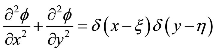 (2.1)
(2.1)
where z is the coordinate of field point P defined as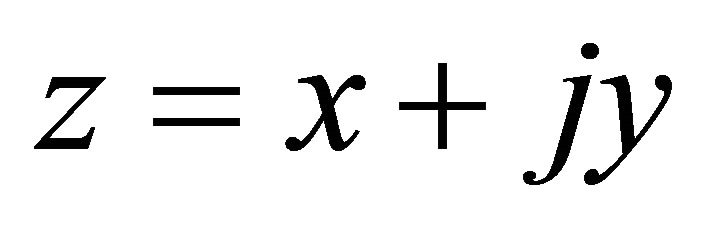 ,
, ; complex number
  is the coordinate of source point Q defined as
 ,
, ; The right of the equation is the product of two delta functions.
The boundary condition on the free surface is:
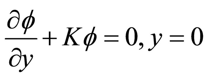 (2.2)
(2.2)
where K,  are real numbers and
  is the unit imaginary number.
At infinite, take the radiation conditions are:
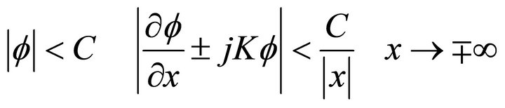 (2.3)
(2.3)
where C is constant.
Ricardo [4] obtained the Green function with the above free surface linear boundary conditions using Fourier transform method:

It can be represented as the following patterns after simplification
 (2.4)
(2.4)
where

and 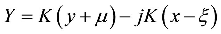 (2.5)
(2.5)
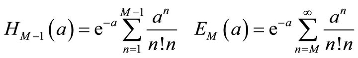
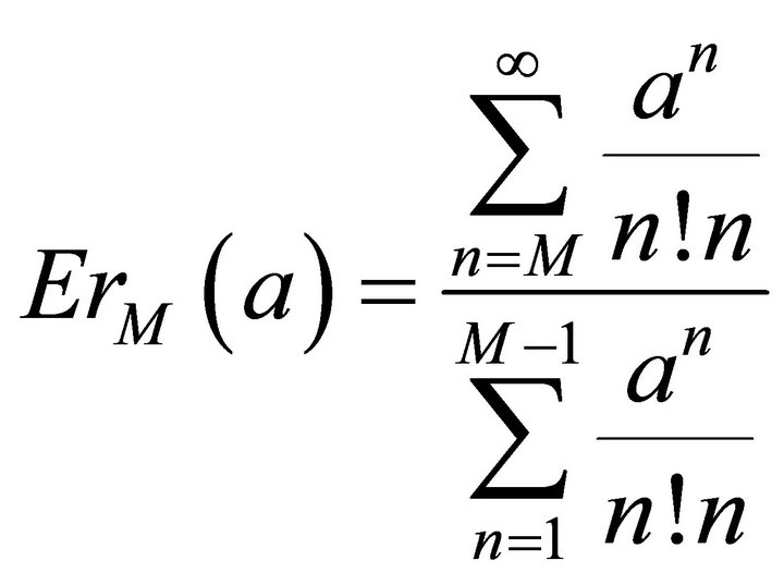
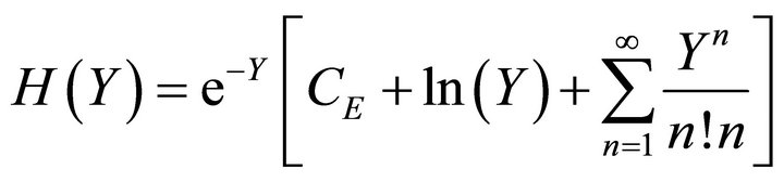
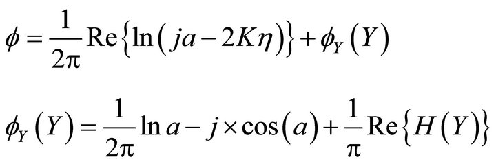
H function is defined as:
 (2.6)
(2.6)
here C is the Euler’s constant. The above formula has only one infinite series, whose denominator is (n!n) and as a result the convergence rate is relatively fast.
3. The Truncation Error of Series
Suppose a and δ is Y’s modulus and argument respectively, When δ is zero, H(Y) proposed above is
 (3.1)
(3.1)
or written as
 (3.2)
(3.2)
where
 (3.3)
(3.3)
Let the relative error noted as
 (3.4)
(3.4)
thus we have
 (3.5)
(3.5)
Since constant a > 0, note q = a/M, then here’s the estimating formula for error

So we get
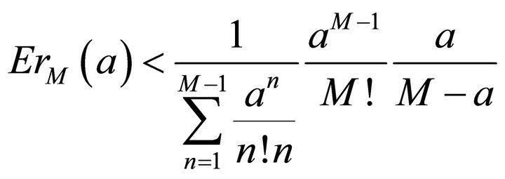 (3.6)
(3.6)
This is the estimating formula for error. Once the positive integer M is given, we can work out the estimated error. On the contrary, if the bound on error is given, we can get the value of M. Assuming the bound on error is 0.01, here’s the relationship of M and a. See details in Table 1.
4. Numerical Calculation
As long as the number of terms in series M is known, we can calculate the values of H(Y) and the Green function based on the proposed formula before. The specific calculation steps are:
1) Give the bound on error;
2) Work out the number of terms in series M;
3) Calculate H(Y) using the following formula
 ;
;
4) Calculate the Green function using the following formula
 .
.
According to these steps, we obtain the real and imaginary part of H(Y). See details in Figure 2, where the pa-
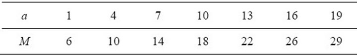
Table 1. Relationship of M (number of terms in series) and a (bound on error).
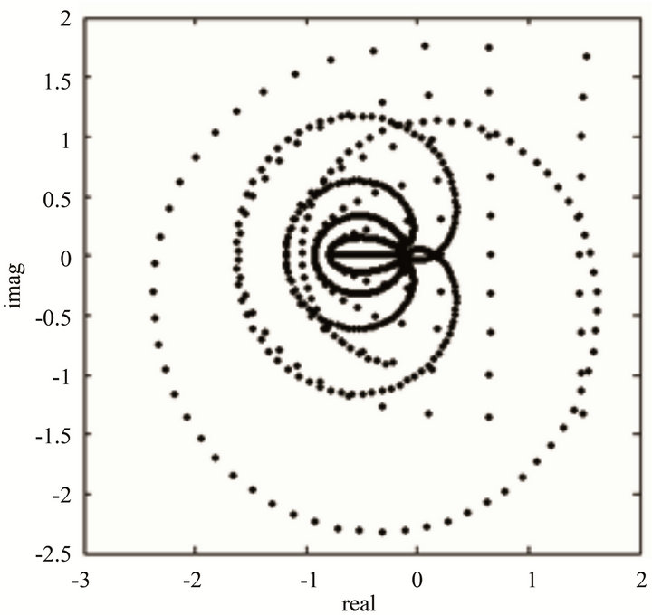
Figure 2. The imaginary part of function H varying with the real part.
rameters’ values are: ;
; ,
, .
.
5. Inherent Properties of the Green Function
We have already got the expression of the Green function, namely

It’s easy to compute the Green function’s first item for its simple logarithmic form. And as a function of complex parameter Y,  can be pre-computation shown by a graph or a table. When Y takes different values, we get these inherent properties.
Property 1: when the argument equals zero, Y = a, and the calculation equation is:

Property 2: when the argument equals 0.5 p, Y = ja, and the calculation equation is:
Property 3: When the modulus of Y tends to infinite, the Green function tends to zero.
6. Conclusion
This paper works out the explicit formulation of the Green function, estimates the formulation’s error and gives the relationship between the number of terms in series M and the bound on error a. Then, inherent properties of the Green function are concluded.
7. Acknowledgements
The paper is financially supported by China national natural science foundation (No. 51139005), and (No. 51279149) and JWSL [2011] 1568).
NOTES
#Corresponding author.