The Optimal Tax Rate: An Empirical Assessment in Congo

Toussaint Armel Bakala

Laboratory of Economics and Management (LEM), Faculty of Economic Sciences, National School of Administration and Magistracy (ENAM), Marien Ngouabi University, Brazzaville, The Republic of Congo.

DOI: 10.4236/ojbm.2024.122058                

Abstract

This article is intended to be an empirical assessment of the optimal tax rate in Congo. The objective pursued by this research work is to determine this optimal tax rate and, therefore, to check whether there is a gap between the effective tax rate and the optimal tax rate, in which case, a correction through fiscal policy is necessary. By adapting Armey’s model to the context of the Congolese economy, it turned out that the optimal tax rate is 17.20%, well below the effective tax rate of 22.5% of non-oil GDP. If the latter seems more in line with the indicators of the Millennium Development Goals (MDGs) and the Sustainable Development Goals (SDGs), it nevertheless appears prohibitive, because it is likely to generate distortions greater than the positive externalities of public expenses.

Keywords

Optimal Tax Rate, Effective Tax Rate, Public Spending, Republic of Congo

1. Introduction

Significant fluctuations in oil prices since the start of the second half of 2014 have considerably affected the economic growth of developing countries whose GDP level essentially depends on oil resources. The need to attract investment and increase non-oil tax revenues has given renewed interest in assessing the optimal tax rate in these developing countries. In the literature, the determination of the optimal tax rate is based on the theory of optimal taxation. This theory studies the taxation system that minimizes economic distortions and inefficiencies. Indeed, the application of taxation generates economic distortions, because economic agents react and modify their behavior. From a theoretical point of view, optimal taxation is based on competitive equilibrium, and therefore relies on the Pareto optimum. Under these conditions, only the flat-rate income tax could be qualified as the first-rate optimum (Mirrlees, 1971) . Indeed, flat-rate taxes are non-distortive in the sense that they depend neither on income, nor on consumption, nor on the choice of factors and in no way modify the decisions of agents and their reasoning at the margin.

Despite everything, the flat-rate tax does not comply with the conditions of equity, which is why the theory of optimal taxation would tend to call into question its applicability. Since the first-rate optimum cannot be achieved through the flat-rate tax, the theory of optimal taxation focuses on the search for a second-rate optimum through the optimal taxation of goods (Ramsey, 1927) and income (Mirrlees, 1971) . Still, taxation is not limited to property and income. It can be extended to capital. We can then speak in terms of overall tax pressure.

The results of studies on determining the optimal tax rate within countries lead to different rate levels depending on the economic structure of the countries studied (Ghossoub Sayegh, & Hamdan Saade, 2020) . As such a study has not yet been carried out in Congo. It is therefore interesting to determine, after an in-depth analysis of the data, an optimal tax rate corresponding to the economic structure of Congo. Also, we will check at the same time, if the tax pressure in Congo is currently below or above the tax rate that tax theory would qualify as optimal.

The relevance of determining an optimal tax rate comes from the fact that it maximizes not only the rate of economic growth (Barro, 1990, 1996; Scully, 1996, 2003) , but also the level of tax revenue. The economic literature recognizes that a certain taxation threshold is necessary for economic viability (Ghossoub Sayegh & Hamdan Saade, 2020) . It is therefore not uninteresting to question the impact of the tax rate in each country, on its economic growth and on the performance of its tax system.

Based on the conclusions of the World Bank on the assessment of the business climate (Doing Business), the high tax burden is one of the disincentivizing factors for investment in the countries of Africa south of the Sahara (ASS). It turns out that, in the “Doing Business 2019” report, Congo ranks 180^th of 189 countries. We can therefore hypothesize that the effective tax pressure in Congo, estimated at 20.12%, does not correspond to its optimal tax rate, and that it is therefore above of the last.

We know, following Vito and Howell (2001) , that determining the optimal tax rate amounts to determining the optimal size of the State. Thus, on a methodological level, relying on the theoretical corpus of optimal taxation (Laffer, 1981; Ramsey, 1927; Mirrlees, 1971) , we will use the quadratic model of Vedder and Gallaway (1998) to determine the rate optimal taxation for the Congo. Then, this optimal tax rate will be compared with the effective tax pressure over recent years.

The rest of this article is organized as follows. We will begin with a review of both theoretical and empirical literature. Next, we will present the stylized facts, and we will continue with an estimation model and its specification. Finally, we will discuss the estimation results before concluding this article.

2. Literature Review

The entire theory relating to the determination of the optimal tax rate mainly revolves around two main axes: optimal taxation and the optimal size of the State.

After having outlined the main theories of optimal taxation, the results of empirical work studying optimal taxation will be reviewed.

2.1. Theoretical Literature on Optimal Taxation

Theories on optimal taxation revolve around three fundamental theories: the Ramsey rule, optimal income taxation and the Laffer theory.

2.1.1. The Theory Based on Ramsey’s Rule

The first theory of optimal taxation is based on the Ramsey rule (Ramsey, 1927) . This theory was developed within the framework of a tax system maximizing efficiency under the assumption that markets are competitive and without externalities. Ramsey’s approach advocates taxing different goods in inverse proportion to the compensated elasticity of supply and demand. It therefore recommends applying low tax rates to goods for which demand is elastic and high rates to those for which demand is inelastic. In other words, according to this theory, to minimize deadweight loss (increase efficiency), one must tax where supplies and demands are least price sensitive; the objective therefore being to create as little distortion as possible. This rule of inverse elasticity leads to an increase in tax pressure on the budgets of poor households. Likewise, such a tax system is unfair because it taxes more those who are not very responsive to taxes: labor more than capital, health expenses, everyday consumer products.

2.1.2. The Theory of Optimal Income Taxation

Several works on optimal taxation (Diamond & Mirlees, 1971a, 1971b) focus on the income tax which is the most redistributive. The objective of redistribution leads to taxing individuals with the highest marginal productivity. This incentivizes individuals with high marginal productivity to reduce labor supply and leads to lower tax revenues. The effect of redistribution on social welfare must then be compared to the effect on the labor supply of high-productivity individuals and on lost tax revenue. These arbitrations make it possible to find an optimal tax rate. This is the rate that should not be exceeded. This rate can be determined by threshold effect models.

Concretely, the theory of optimal income taxation aims to clarify the determinants of an optimal tax scale. On the one hand, a progressive scale, that is to say where the level of the tax rate increases with the level of income and thus leads to gains in terms of equity. On the other hand, such a scale creates distortions in the labor supply by discouraging individuals from making more effort. Such discouragement can be circumvented by practicing tax avoidance behavior, also called tax avoidance behavior. These types of behavior manifest themselves through tax evasion and tax optimization. The two types of behavior are similar because they both cause losses in tax revenue. However, they differ in that tax fraud consists of a violation of tax law while tax optimization is the circumvention of tax law by taking advantage of loopholes in tax law or even legal loopholes.

One of the most important conclusions of Mirrlees’s (1971) work is that marginal tax rates should be lower as income increases.

2.1.3. Laffer’s Theory

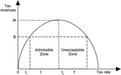
The third theory of optimal taxation is that of the supply theorists, resulting from the CJL model (Canto, Joïnes and Laffer) which resulted in the Laffer curve (Laffer 1981) ¹. The latter is often summarized by the formula “Too much tax kills tax”. Indeed, increasing the rate of compulsory deductions up to a certain threshold generates an increase in revenue, beyond this threshold, tax revenue decreases because active workers will prefer leisure to work. The supply of labor and capital decreases with the increase in the marginal tax rate. To reverse such a trend, public spending must be reduced and the rate of compulsory contributions must be reduced. Indeed, Laffer’s idea is to show that beyond a certain threshold, any increase in the tax rate (noted t) paradoxically causes a drop in the total amount of tax revenue.

Tax revenue is first an increasing function of the tax rate, until reaching a maximum threshold M (top of the curve); beyond M, tax revenues are a decreasing function of the tax rate. This means that the same level of tax revenue can be obtained by two different tax rates (respectively t₁ and t₂) located on either side of the optimal rate (t*). The zone between 0 and t* is described by Laffer as an “admissible zone” or zone of increasing returns, while beyond t* it is an “unacceptable zone” or zone of diminishing returns.

Here we use microeconomics with the notions of income effect and substitution effect to explain the evolution of the Laffer curve. The increase in the tax rate has two effects on an agent’s choice between working time and leisure time:

· a substitution effect: if t increases, disposable income decreases; work is in some way penalized, which encourages the agent to reduce their working time and increase their leisure time;

· an income effect: if t increases, disposable income decreases, which can encourage the agent to work more to regain his initial income.

The final impact of an increase in the tax rate on labor supply will therefore depend on the magnitude of these two effects. According to Laffer, for high rates, the substitution effect would outweigh the income effect, which would lead to a reduction in the overall amount of expected tax revenue; the Laffer curve shows precisely that beyond t*, the tax base contracts more quickly than the increase in the rate of tax pressure.

The substitution effect can be extended to the arbitration between declared work and “black work”: when the tax rate increases, the agent tends to resort more and more to the underground economy. Likewise, the substitution effect can relate to the trade-off between the market economy and the domestic economy: figuratively, an increase in the tax rate encourages people to cultivate their vegetable garden rather than working to buy vegetables at the market. In reality, what is true for the supply is also true for the supply of capital: if savings are heavily taxed, individuals are encouraged to consume rather than accumulate capital, which determines tax revenue, through investments and therefore economic growth.

Laffer’s theory is rather part of the analysis of the overall tax burden of an economy. However, Laffer only takes up an old idea, already exposed by Khaldoun (1377) , Dupuit (1844) . The Laffer curve has been the subject of several criticisms: first of all, the existence of a “kinked” labor supply curve remains controversial. Indeed, in the short term, given the constraints faced by the agent (rent, loans to repay, etc.), a reduction in the salary tax rate is more likely to lead to an increase in the supply of work.

Then, the Laffer curve is a partial reasoning since it only perceives the tax at the microeconomic level as being a drain; however, at the macroeconomic level, tax is the origin of public expenditure. Indeed, it takes into account neither the welfare costs of the tax nor the marginal utility of the financed expenditure. It is ultimately limited to justifying why governments should ease the tax burden.

Finally, being part of the supply side only, the CJL model ignores the effects of demand, that is to say the income effect of tax policy through redistribution.

2.2. Literature on Optimal Tax Rate Evaluation Models

Given that determining the optimal tax rate amounts to determining the optimal size of the State (Vito & Howell, 2001) , certain evaluation models favor the determination of the optimal tax rate, and others, the size optimal state. The literature in this area identifies five main models for evaluating the optimal tax rate: the Barro model (Barro, 1991) , the Armey model (Armey, 1995) , the Scully model (Scully, 1996, 2003) , and that of Vedder and Gallaway (1998) and the threshold effect models of Hansen (1999, 2000) and Caner and Hansen (2004) .

First, from a long-term perspective and through his modeling of productive public expenditure, Barro (1991) integrates the active role of government policy into a standard endogenous growth model of Rebelo (1991) . This model, based on a single sector, has the advantage of treating in a unified framework both the positive effect of public spending and the negative effect of income taxation. In other words, this model of endogenous growth with externalities of public spending (infrastructure for example) accounts for the non-linear relationship between taxation and growth. Indeed, an increase in the tax rate provides resources to finance productive public spending, but at the same time reduces the net marginal return on private capital. This trade-off leads to a threshold effect in the relationship between public spending and long-term growth. This therefore results in an optimal level of productive public spending which is equivalent to the optimal size of the State.

Barro’s model (Barro, 1990) assumes that the state budget is balanced. This hypothesis is contrary to empirical observations, since public deficits do not cancel out, on average, over very long periods (Villieu, 2015) . Formally, the hypothesis of a long-term balanced budget is justified in a model without growth (Villieu, 2015) .

Following Barro (1991) , Armey (1995) proposed a model based on an inverted U curve, similar to that of Laffer (1981) to represent the effects of public expenditure on national income. Armey relied on the idea that when government spending is low, the growth rate of the economy is also low. On the other hand, when the level of public spending is very high, the weight of the State in the economy may appear excessive: such a situation diverts too large a quantity of wealth for the benefit of the State, thus penalizing the private sector which no longer has sufficient resources to stimulate economic growth. There is therefore a threshold for public spending below which it has a positive effect on growth and beyond which the effect would be negative on growth. Then, Scully (1998) using a two-sector model, showed that the more the size of the State increases as a percentage in an economy, the more economic growth decreases significantly, because resources are used less efficiently. The author places the optimal size of the State at approximately one fifth of the size of a country’s economy. The Scully model is considered an alternative to the Barro optimal tax rate model, since it also determines a relationship between the level of taxation and growth.

Regarding the Vedder and Gallaway (1998) model, the authors highlight Armey’s theoretical approach. The model of these authors ensures the prevalence of a quadratic relationship between economic growth and the rate of tax pressure.

Finally, for models with a threshold effect, we distinguish the model of Hansen (1999, 2000) for which the threshold variable is endogenous and that of Caner and Hansen (2004) , where the threshold variable is exogenous. Both types of model determine a threshold tax rate, below which tax revenues gradually increase and above which tax revenues gradually fall.

2.3. Some Empirical Work

Empirically, research focuses on determining the optimal tax rate, and on determining the optimal level of public spending. Concerning the work on determining the optimal tax rate, Colin Clark (1940) showed that the tax levy should not exceed a quarter (25%). The Physiocrats, on the other hand, believe that this threshold would be around 20%.

Scully (1996, 2003) highlighted the existence of an inverted U-shaped relationship in the case of New Zealand over the period from 1927-1994. It obtains a tax rate that maximizes the growth rate of around 20% of GDP. Another study carried out by Scully (1995) estimated the optimal rate of tax pressure for the United States, between 21.5% and 22.9% of GDP over the period from 1949 to 1989, then at 21% of GDP over the period from 1950 to 1995. The author obtains the rate of 34.1% for the United Kingdom and 51.6% for Denmark.

Saibu (2015) empirically determines the optimal tax rate for Nigeria and South Africa. He rejects the hypothesis of non-linearity of the effects of the tax, in the context of South Africa, while a significant non-linear relationship is observed in the case of Nigeria. Its results lead to an optimal tax rate of around 15% of GDP per capita for South Africa and 30% for Nigeria. Within the framework of the West African Economic and Monetary Union (UEMOA), for the period from 1980 to 2016, using a Scully optimization model and a quadratic model, is reached the optimal rate of 21.04% and 23.8% respectively.

Fölster and Henrekson (1999) ; Karras (1999) ; Blanchard and Perotti (2002) ; Romer and Romer (2007) ; Favero and Giavazzi (2009) analyzed the link between taxes and economic growth. The results obtained, however, are quite mixed since they vary from one country to another. As for the optimal level of debt, a study conducted by Tanimoune et al. (2005) , showed that for UEMOA countries the optimal level of debt is 83%.

Regarding the work focused on determining the optimal level of public spending, a study carried out by Illarionov & Pivarova (2002) for the period from 1960 to 2000 came to the conclusion that, the increase in A percentage point in the share of public spending in relation to GDP is accompanied by a reduction of 0.1% in the average growth rates of economic activity. Pevain seeks proof of the phenomenon of Armey (1995) in twelve European countries over the period 1950-1996: the results obtained by the author show the decrease in the marginal productivity of public spending as soon as the threshold of 37.09% is reached.

Forte & Magazzino (2010) show the existence of the Armey curve in 27 countries of the European Union using a dual estimation technique using panel data and time series over the period from 1970 to 2009. They obtain the optimal level of public spending of around 37% on average.

In light of the above, the results on the optimal tax rate obtained differ depending on the countries, the periods of study, the source of the data, the methodology used and the tax variables retained (Ghossoub Sayegh & Hamdan Saade, 2020) .

3. Stylized Facts

The GDP growth rate between 1987 and 2017 is quite volatile, it varies between −5.49% and 8.75% (see following graph). Several factors are likely to impact the stability of the growth rate, among which is the level of the tax rate.

The evolution of the curves of the economic growth rate (Graph 1) and the overall tax rate (Graph 2) suggests the presence of a “Laffer growth curve”, which therefore assumes a cyclical relationship between the rate of economic growth and the tax rate in the long term. The juxtaposition of these curves shows that on average phases of decline in economic growth follow phases of increase in tax rates.

The graph below shows that the relationship between the tax rate and the growth rate takes the form of an inverted U (Graph 3), which indeed seems to confirm our intuition about the existence of a growth Laffer curve.

Graph 1. Evolution of the growth rate from 1987 to 2017. Source: author based on World Bank data.

Graph 2. Evolution of the overall tax rate from 1987 to 2017. Source: author based on BEAC data.

Graph 3. Non-linear evolution of the overall tax rate and the growth rate from 1987 to 2017. Source: author based on data from the World Bank and the BEAC.

4. Determination of the Estimation Model

We use Armey’s model (Armey, 1995) and adapt it to the context of the Congolese economy.

In order to identify the inflection point of the Armey (1995) curve of public expenditure and their components in relation to GDP per capita, we will use a quadratic specification following the example of Armey (1995) :

${\text{GDP}}_{/pc}=a+b{G}_{it}-c{G}_{it}^2+dT+e{K}_{it}+{\text{ω}}_{it}$ (1)

With:

${\text{GDP}}_{/pc}$ , represents the growth rate of GDP per capita.

G² is assumed to be negative in sign and thus measures the opposite effect associated with increasing the level of public spending beyond the optimal threshold. In other words, this term indicates the decrease in the marginal productivity of public spending. If the value of the squared term grows faster than the value of the linear term then the negative effect of public spending outweighs the positive effect of it. By analogy, this hypothesis will be applied to the components of public expenditure. T is a time variable representing the development of human capital and resources over time (value 1 for the first year, value 2 for the second year, so on, etc.); K, represents certain variables retained (imports, exports, public spending, gross private capital formation), and ω, is the error term.

4.1. Model Specification

Our Armey model (Armey, 1995) adapted for the Congo is presented as follows.

${\text{LGDP}}_t={\text{α}}_0+{\text{α}}_1{\text{EXP}}_t+{\text{α}}_2{\text{PE}}_t+{\text{α}}_3{\text{GPFCF}}_t+{\text{α}}_4{\text{TR}}_t+{\text{α}}_5{\text{TR}}_t^2+{\text{μ}}_t$ (2)

With:

LPIB: Logarithm of non-oil GDP; EXP: Export; PE: Public Expenditure; GPFCF: Gross private fixed capital formation; TR: The tax rate or tax pressure excluding oil; TR²: The squared tax rate excluding oil; TR*: Optimal tax rate excluding oil. The tax threshold is obtained by deriving Equation (2) in relation to the tax pressure variable

$\begin{array}{l}{\text{TR}}^{\ast }=\frac{\Delta \left(\text{LGDP}\right)}{\Delta \left(\text{TR}\right)}=0\\ \Rightarrow \frac{\Delta \left({\text{α}}_0+{\text{α}}_1{\text{EXP}}_t+{\text{α}}_2{\text{PE}}_t+{\text{α}}_3{\text{GPFCF}}_t+{\text{α}}_4{\text{TR}}_t+{\text{α}}_5{\text{TR}}_t^2+{\text{μ}}_t\right)}{\Delta \text{TR}}=0\end{array}$

${\text{α}}_4+2{\text{α}}_5\text{TR}=0\Rightarrow 2{\text{α}}_5\text{TIM}=-{\text{α}}_4$

${\text{TR}}^{\ast }=\frac{-{\text{α}}_4}{2{\text{α}}_5}$ (3)

It is the rate that optimizes economic growth.

4.2. Estimation of the Model

Let us first present the sources and describe the data before proceeding to the discussion of the results.

4.2.1. Data Sources and Description of Variables

Let us present the data sources, before proceeding to describe the variables.

· Data sources

It should be noted that annual data have been transformed into quarterly data (1987.Q4-2017.Q1). In fact, the series studied is annual while the model which will reproduce it must generate quarterly data. To achieve this, we used Denton’s quarterly method (Denton, 1971) , which is the method most used by IMF economists.

· Description of variables

Exports (EXP) are taken into account in our model because they constitute a component of overall demand. Its increase has a multiplier effect on non-oil GDP. However, in economies dependent on oil exploitation, an increase in the value of exports resulting from an increase in the price of a barrel of oil can be unfavorable for activities in the non-oil sector. This fact can be explained by the “Dutch disease”. To this end, the expected effect of an increase in exports on non-oil GDP is therefore nuanced. Public spending (PE) has a positive effect on growth if the effect of positive externalities generated by public spending is greater than that of the distortions created by taxation. In the opposite case, public spending has a negative effect on growth. This negative effect of public spending is further reinforced if unproductive spending² takes up a significant share of total public spending. The gross formation of private fixed capital (GPFCF) also has a positive effect on growth, because the increase in investment increases the production capacity of companies, as a result, production increases. Also, the gross formation of fiscal capital is a component of overall demand, its increase leads to an increase in non-oil GDP.

The tax rate is the ratio between non-oil tax revenue and non-oil GDP, in other words tax pressure rate. The (TR)² is generated from the tax pressure rate. Taking into account the TR and (TR)² is justified by the existence of a non-linear relationship between the tax rate and non-oil growth. Based on the approach of Barro (1990) which recognizes the existence of a threshold effect between the tax rate and the non-oil growth rate, we assume that the rate of tax pressure first of all, can have a positive effect on growth but beyond a certain threshold the increase in the tax rate reduces non-oil growth. In this case, the expected sign of the tax rate will be positive, while that of the squared tax rate (TR)² will be negative, such that an optimal tax rate results.

4.2.2. Estimation Results

Let us proceed to determine the order of integration of the variables, the optimal delay and the rank of cointegration of the variables, the estimation of the error correction model and the discussion of the results.

Variable stationarity test

To study the stationarity of the variables, we carried out the Augmented Dickey and Fuller, Phillip Perron and Kwiatkowski-Phillips-Schmidt-Shin tests using the Eviews software. The results of these tests are summarized in Table 1.

The results of these different tests show that the variables of our study are all integrated of order 1 [I (1)], which leads us to determine the cointegration rank of the variables. However, before determining the cointegration rank, it is first necessary to know the optimal lag number.

Optimal number of lags and variable cointegration test

An important step in the context of dynamic models is the determination of the optimum number of delays to consider. To determine it, different criteria are often used, the most common of which are: Akaike Information Criterion (AIC) and Schwartz Information Criterion (SIC). If applicable, the test indicates the existence of two delays by the AIC and SIC criteria. Thus, the delay number 2 is retained. This is summarized in Table 2 (see appendix, Optimal Lag).

The results of the Johansen cointegration test reported in this table show that all the variables are integrated of order 1. The results of the cointegration rank of the variables will be represented in Table 3.

Thus, the application of the error correction model seems to be appropriate in the context of our work.

The estimation results of the error correction model

The results of estimating the Laffer curve of growth can be summarized in Table 4 below.

The results of our estimations show that the error correction coefficients [Cointeq(-1) and Cointeq(2)] are negative and significant at the 1% level, thus proving the validity of the error correction model. Also, the R² is equal to 0.669436 or 66.94% and the adjusted R² is equal to 0.620823 or 62.08%.

Table 1. Determination of the order of integration of variables.

Source: author from Eviews.

Table 2. Determination of the optimal delay.

Source: author from Eviews software.

Table 3. Results of the cointegration rank of the variables.

Source: author from Eviews.

Table 4. MCE result.

Source: author based on results (appendix, Test on model residuals).

Such an observation suggests that economic growth is explained by the exogenous variables retained. The ARCH test shows that the probability of “Obs*R-squared” is equal to 0.9051, greater than 5%. We accept the null hypothesis of homocedasticity of the residuals. The Breusch-Godfrey test allows us to accept the hypothesis of homocedasticity of errors, because the relative probability is equal to 0.527399, greater than 5%; the probability associated with the Breusch-Pagan-Godfrey test is 0.2293 and this probability reveals that there is no correlation of errors. Finally, the model stability tests, Cusum and Cusum squared, show that the model is structurally and punctually stable.

5. Discussion of Results

The results show that the tax rate (TR) has a positive effect on non-oil growth. Indeed, an increase in the tax rate of 1% leads to an increase in non-oil growth of 0.0184%. While an increase in the squared tax rate (TR²) of 1% induces a reduction in non-oil growth of 0.00053%. This results in an optimal tax rate of 17.20%. In accordance with the Laffer curve, our results show that an increase in the tax rate leads to an increase in economic growth, but beyond 17.20% any increase in the tax rate leads to a decrease in growth. In terms of tax yield, below this threshold rate, tax revenue increases but above this threshold rate, tax revenue falls. This optimal rate is below the average tax rate from 1987 to 2017 which stands at 20.12%. This therefore results in tax avoidance behavior in Congo. It can therefore be recommended, as part of its economic policy, that the Congo lower its effective pressure rate to around 17% to expect an increase in economic growth and an increase in tax revenue. The optimal tax rate obtained for the case of Congo is consistent with that required by the second-tier convergence criteria of CEMAC. However, the effective tax rate is close to that recommended by the MDGs and SDGs as a necessary threshold for financing development. The rate recommended by the MDGs and SDGs is prohibitive and is likely to generate distortions which will be greater than the positive externalities of public spending.

Our results are in line with those of Keho (2010) , Motloja (2016) , Salaheddine & Abdellah (2018) and Yawovi (2018) , who showed the existence of a Laffer curve of growth, respectively in Côte d Ivory, in South Africa, Morocco and in UEMOA countries.

A positive effect is observed in the response of growth to an increase in public spending, since our model shows that a 1% increase in public spending causes an increase in growth of 0.0088%. Indeed, an increase in unproductive public spending (public consumption) leads to an increase in demand. However, as production capacity is limited, imports increase more quickly, the positive effect on growth is therefore just as limited.

As for the gross formation of private fixed capital, its effect on economic growth also turns out to be positive, because an increase of 1% in the gross formation of private fixed capital leads to an increase of 0.0011%. Indeed, an increase in the gross formation of private fixed capital results in an increase in the production capacity of companies, and consequently, an increase in production.

6. Conclusion

The objective of this research was to determine the optimal tax rate in Congo in order to compare it with the effective rate of compulsory levies. Using the Armey model that we adapted to the Congolese context, the estimates gave an optimal tax rate of 17.20%. This rate is well below the effective tax rate which is around 22.52% of non-oil GDP. The difference between these two rates suggests a downward correction of the tax pressure, and therefore the implications for economic policy.

An important limitation of this research work results from the fact of not having determined the optimal tax rates by type of tax, relying of course on the Ramsey rule (Ramsey, 1927) and the optimal income taxation of Mirrlees (1971) . Thus, determining an optimal tax rate by type of tax may be the subject of other future research work.

Appendices

Stationarity Test

Augmented Dickey-Fuller

*MacKinnon (1996) one-sided p-values.

*MacKinnon (1996) one-sided p-values.

*MacKinnon (1996) one-sided p-values.

*MacKinnon (1996) one-sided p-values.

*MacKinnon (1996) one-sided p-values.

*MacKinnon (1996) one-sided p-values.

*MacKinnon (1996) one-sided p-values.

*MacKinnon (1996) one-sided p-values.

*MacKinnon (1996) one-sided p-values.

*MacKinnon (1996) one-sided p-values.

*MacKinnon (1996) one-sided p-values.

*MacKinnon (1996) one-sided p-values.

Optimal Lag

*Indicates lag order selected by the criterion; LR: sequential modified LR test statistic (each test at 5% level); FPE: Final prediction error; AIC: Akaike information criterion; SC: Schwarz information criterion; HQ: Hannan-Quinn information criterion.

Testing Model Residuals

NOTES

¹In fact, the Laffer curve appeared in 1977 but was the subject of a publication in a Scientific Journal in 1981.

²This is the case for expenditure linked to interest on the public debt.

Conflicts of Interest

The authors declare no conflicts of interest.

References

[1]	Armey, D. (1995). The Freedom Revolution. Regnery Publishing.
[2]	Barro, R. J. (1990). Government Spending in a Simple Model of Endogenous Growth. Policy Economics, 98, 103-125. https://doi.org/10.1086/261726
[3]	Barro, R. J. (1991). Economic Growth in a Cross Section of Countries. The Quarterly Journal of Economics, 106, 407-443. https://doi.org/10.2307/2937943
[4]	Barro, R. J. (1996). Determinants of Economic Growth: A Cross Empirical Study (pp. 1-108). Working Paper, NBER. https://doi.org/10.3386/w5698
[5]	Blanchard, O., & Perotti, R. (2002). An Empirical Characterization of the Dynamic Effects of Changes in Government Spending and Taxes on Output. The Quarterly Journal of Economics, 117, 1329-1368. https://doi.org/10.1162/003355302320935043
[6]	Caner, M., & Hansen, B. (2004). Instrumental Variable Estimation of a Threshold Model. Econometric Theory, 20, 813-843. https://doi.org/10.1017/S0266466604205011
[7]	Clark, C. (1940). The Conditions of Economic Progress. Macmillan, 504 p.
[8]	Denton, F. (1971). Adjustment of Monthly or Quarterly Series to Annual Totals: An Approach Based on Quadratic Minimization. Journal of the American Statistical Association, 66, 99-102. https://doi.org/10.1080/01621459.1971.10482227
[9]	Diamond, P., & Mirlees, J. (1971a). Optimal Taxation and Public Production I: Production in Efficiency. American Economic Review, 61, 8-27.
[10]	Diamond, P., & Mirlees, J. (1971b). Optimal Taxation and Public Production II: Tax Rules. American Economic Review, 61, 261-278.
[11]	Dupuit, J. (1844). De la mesure de l’utilité des travaux publics. Revue Française d’économie, 10, 55-94. https://doi.org/10.3406/rfeco.1995.978
[12]	Favero, C. A., & Giavazzi, F. (2009). How Large Are the Effects of Tax Changes? NBER Working Paper, No. 15303, National Bureau of Economic Research. https://doi.org/10.3386/w15303
[13]	Fölster, S., & Henrekson, M. (1999). Growth and the Public Sector: A Critique of the Critics. European Journal of Political Economy, 15, 337-358. https://doi.org/10.1016/S0176-2680(99)00010-5
[14]	Forte, F., & Magazzino, C. (2010). Optimal Size of Government and Economic Growth in the EU-27. Working Papers 0410, CREI L’Università degli Studi Roma Tre, Revised 2010.
[15]	Ghossoub Sayegh, R., & Hamdan Saade, N. (2020). Optimal Tax Rate and Economic Growth: An Empirical Application to the Case of Lebanon. International Review of French-Speaking Economists, 5, 66-86. https://doi.org/10.18559/RIELF.2020.2.3
[16]	Hansen, B. E. (1999). Threshold Effects in Non-Dynamic Panels: Estimation, Testing and Inference. Journal of Econometrics, 93, 334-368. https://doi.org/10.1016/S0304-4076(99)00025-1
[17]	Hansen, B. E. (2000). Sample Splitting and Threshold Estimation. Econometrica, 68, 575-603. https://doi.org/10.1111/1468-0262.00124
[18]	Illarionov, A., & Pivovarova, N. (2002). The Size of Government and Economic Growth. Voprosy Ekonomiki, 9, 18-42.
[19]	Karras, G. (1999). Taxes and Growth: Testing the Neoclassical and Endogenous Growth Models. Contemporary Economic Policy, 17, 177-188. https://doi.org/10.1111/j.1465-7287.1999.tb00673.x
[20]	Keho, Y. (2010). Estimating the Growth-Maximizing Tax Rate for Cote d’Ivoire: Evidence and Implications. Journal of Economics and International Finance, 2, 164-174.
[21]	Khaldoun, I. (1377). Discourse on Universal History. Al-Muqaddima (Translation from Arabic by Vincent Monteil). Lebanese Commission for the Translation of Masterpieces, 1967-1968, 1132 p.
[22]	Laffer, A. B. (1981). Supply Side Economics. Financial Analyzes Journal, 37, 29-44. https://doi.org/10.2469/faj.v37.n5.29
[23]	Mirrlees, J. A. (1971). An Exploration in the Theory of Optimum Income Taxation. The Review of Economic Studies, 38, 175-208. https://doi.org/10.2307/2296779
[24]	Motloja, L. A. (2016). Changes in the Optimal Tax Rate in South Africa Prior and Subsequent to the Global Recession Period. Department of Economics (pp. 2-17). Finance and Business Studies, CTI Potchefstroom Campus, North West, South Africa.
[25]	Ramsey, F. (1927). A Contribution of the Theory of Taxation. Economic Journal, 37, 47-61. https://doi.org/10.2307/2222721
[26]	Rebelo, S. (1991). Long-Run Policy Analysis and Long-Run Growth. Journal of Political Economy, 99, 500-521. https://doi.org/10.1086/261764
[27]	Romer, C. D., & Romer, D. H. (2007). The Macroeconomic Effects of Tax Changes: Estimates Based on a New Measure of Fiscal Shocks. NBER Working Paper No. 13264, 71 p. https://doi.org/10.3386/w13264
[28]	Saibu, O. M. (2015). Optimal Tax Rate and Economic Growth. Evidence from Nigeria and South Africa. EuroEconomica, 1, 41-50.
[29]	Salaheddine, S., & Abdellah, E. (2018). Modeling the Optimal Tax Pressure in Morocco. International Journal of Advanced Research, 6, 136-156.
[30]	Scully, G. W. (1995). The Growth Tax in the United States. Public Choice, 85, 71-80. https://doi.org/10.1007/BF01047902
[31]	Scully, G. W. (1996). Taxation and Economic Growth in New Zealand. Pacific Economic Review, 1, 169-177. https://doi.org/10.1111/j.1468-0106.1996.tb00182.x
[32]	Scully, G. W. (1998). Measuring the Burden of High Taxes. Policy Report No. 215, National Center for Policy Analysis.
[33]	Scully, G. W. (2003). Optimal Taxation, Economic Growth and Income Inequality. Public Choice, 115, 229-312. https://doi.org/10.1023/A:1024223916710
[34]	Tanimoune, N. A. et al. (2005). Les effets non linéaires de la politique budgétaire: Le cas de l’Union Economique et Monétaire Ouest Africaine. Communication aux journées de l’AFSE, Economie du développement et de la transition, Clermont-Ferrand, 19-20 Mai 2005, 24 p.
[35]	Vedder, R. K., & Gallaway, L. E. (1998). Size of Government and Economic Growth. In The Joint Economic Committee of US Congress (pp. 1-15).
[36]	Villieu, P. (2015). Macré Conomie. Ed. Economica, 536 p.
[37]	Vito, T., & Howell, Z. (2001). Tax Policy for Developing Countries (pp. 1-12). International Monetary Fund, Economic Issues No. 27.
[38]	Yawovi, M. I. A. (2018). Review of Optimality of Tax Performance in Developing Countries: Evidence from WAEMU. Université Clermont-Auvergne.