Corruption Perception Index (CPI) in European countries: Monitoring with GIS

Papageorgiou Christos, Dermatis Zacharias, Komninos Dimitrios, Anastasiou Athanasios^*

Department of Management Science and Technology, Laboratory of Data Science and Digital Transformation, University of Peloponnese, Tripolis, Greece.

DOI: 10.4236/tel.[phone]                

Abstract

This paper examines the relationship between corruption and economic growth in European countries, taking into account that corruption is considered as a political, economic, cultural and moral problem. Specifically, this paper will focus on countries of the Eurozone, the European Union, the European Economic Area and the Central and Eastern European countries, including Turkey and Kazakhstan, over the period from 2005 to 2021. Our ultimate goal is to understand how corruption affects economic development by tracking the GDP per capita and the values of measured corruption and also how changes in GDP growth rates are affected by corruption changes. In addition to graphs, the survey provides numerical results displayed in charts using Geographical Information System (GIS). Our survey shows that all European countries with high GDP per capita tend to have low corruption values, with the exception of the countries in Central and Eastern Europe, including Turkey and Kazakhstan. The survey also shows that higher GDP per capita growth rates are correlated linearly with the reduction of the corruption levels in all categories of almost all European countries, with the exception the Central and Eastern European countries, including Turkey and Kazakhstan.

Keywords

Corruption, GDP Per Capita, Economic Growth, European Countries, GIS, Per Capita GDP Growth Rate

1. Introduction—Measuring Corruption

Corruption is measured using questionnaires designed by certain companies. As these questionnaires focus on the experiences of individuals or groups, they contain subjective data. The results of these surveys are published in the form of specific or composite indicators (Mocan, 2008) . Some of these indicators are:

· Every year since 1995, Transparency International organization measured the public’s Corruption Perceptions Index (CPI) as a composite index in each country. This index combines annual data on perceived corruption in the public sector for specific organisations and individuals.

· The World Bank uses a six-monthly survey called the Control of Corruption Index (CCI), which includes data from organisations and individuals outside the World Bank. This index is a composite index that focuses on public corruption.

· Starting from the time period 1981-1983, the Economist Intelligence Unit collects data from around the world on levels of corruption in order to calculate the Business International (BI) index (Economist Intelligence Unit, 2016) .

· Transparency International non-governmental organization publishes the annual Global Corruption Barometer (GCB). The survey examines people’s views on corruption and has been conducted by the organization since 2003.

· Transparency International organization measures the ability of companies to bribe public officials and institutions in countries with less developed economies. The resulting Bribe Payers Index (BPI) is based on surveys of senior business and banking executives conducted by the international non-governmental organisation.

· Political Risk Services Inc. publishes a monthly report on the political and financial risks of more than 140 countries, which analyses each country’s level of risk in both areas using the International Country Risk Guide (ICRG) (Political Risk Services Inc., 2016) .

The Corruption Perception Index (CPI) is based on a survey of businesses and individuals around the world. It consists of twelve sub-indices, which are listed in Appendices. It is considered a composite index because its data come from several surveys—at least three for each country surveyed—and currently these surveys cover 180 countries (Anastasiou & Panagiotopoulou, 2020; Komninos et al., 2020) . The CPI index is based on values between 0 and 100. Before 2011, values between 0 and 10 were used. The value of 0 indicates the maximum corruption, while the value of 100 indicates the sense that there is no corruption at all in the country. This index is used throughout this paper. However the use of this index may create some problems when used as an important criterion for the actual levels of corruption in a country (Malito, 2014) :

· The sub-indices of the final index represent different forms of corruption, as there is no universally accepted definition of corruption. Each sub-index is constructed using a different research methodology.

· Information problems arise because of the different perspectives of different countries. In addition, individuals’ biased opinions flourish.

· Many countries rank higher on a corruption scale because of the value of their index. However, this index is often not comparable with other years’ results.

2. Relating Corruption with per Capita GDP & per Capita GDP Growth

Experts suggest that the growth rate of GDP per capita is the best measure of the economic growth of a country. However, apart from the per capita GDP growth rate of a country, it is also of particular significance whether the per capita GDP converges at some level, determined by the internal factors of a country’s economic policy or by externally imposed criteria set for the country (Anastasiou et al., 2022; Anastasiou et al., 2021) . The basic condition for convergence is the negative relation of the per capita GDP growth rate (g_yi) of the country (i) and the per capita GDP (y_i) of the same country (i). This relationship as a function has the form:

$g_{yi}=f\left(\log y_i\right)$ (1)

where:

g_yi = The per capita GDP growth rate of the country (i)

y_i = The per capita GDP of country (i)

For a constant growth rate ( $g_{yi{t}_1{t}_2}$ ), Equation (1) is written as:

$y_{i{t}_2}=y_{i{t}_1}{\text{e}}^{g_{yi{t}_1{t}_2}\cdot \Delta t}$ (2)

where:

$g_{yi{t}_1{t}_2}$ = The mean per capita GDP growth rate of country (i), during the period of time Δt (where Δt = t₂ – t₁),

$y_{i{t}_1}$ = The initial per capita GDP of country (i) at time (t1)

$y_{i{t}_2}$ = The final per capita GDP of country (i) at time (t2)

And in logarithmic form:

$g_{yi{t}_1{t}_2}=\left(\ln y_{i{t}_2}-\ln y_{i{t}_1}\right)/\Delta t$ (3)

For (t₁ = t) and (t₂ = t + 1), i.e. for a period of time of one year, then Δt = 1 and Equation (3) is written as a logarithmic difference for the estimation of the annual per capita GDP growth rate:

$g_{yit\left(t+1\right)}=\ln y_{i\left(t+1\right)}-\ln y_{it}$ (4)

To take into account socio-economic factors, Barro (Barro, 1991) used an empirical form of Equation (4), which includes a set of variables such as health systems and schools. His equation is as follows (Akçay, 2002) :

$g_{yi{t}_1{t}_2}=a\log y_{i{t}_1}+cX+d$ (5)

where:

X = A group of variables which include socio-economic effects

a, c, d = Constants (α < 0 for the cases of economic convergence)

Mauro (Mauro, 1995) analysed the relationship between corruption and annual economic growth over a period from 1960 to 1985, using data from the BI corruption index for 67 countries for the time period 1980-1983. He found that countries with low levels of corruption had higher average annual growth rates than countries with high levels of corruption. He also found that the improvement of the corruption index had a positive effect on GDP growth and investment. This was largely due to the fact that the improvement of the corruption index by one degree increased GDP per capita by 0.5% and investment by 5% of GDP per year. Using the extended Barro equation (Equation (5)), Mauro (Mauro, 1995) extended the equation to include corruption (Akçay, 2002) :

$g_{yi{t}_1{t}_2}=a\log y_{i{t}_1}+bCo{r}_{i{t}_1}+cX+d$ (6)

where:

$Co{r}_{i{t}_1}$ = Corruption index of country (i) at time (t1)

X = A group of variables which include socio-economic effects

a, b, c, d = Constants (a < 0, b > 0)

Mauro (Mauro, 1998) used the ICRG index for 1982 to 1995 and the BI index for 1980 to 1983. For a sample of 106 countries, he studied the effect of corruption on growth and investment, where the dependent variables were the average rate of investment and GDP growth for each country. Mauro found that countries with improvement of the corruption indices by a single unit, had a 4% higher investment growth rate and a 0.5% higher GDP per capita growth rate, over the time period from 1960 to 1985.

Ehrlich and Lui (Ehrlich & Lui, 1999) found that countries with higher levels of corruption had lower economic growth rates. They studied the data from 152 countries from 1960 to 1992 and found that the higher the level of corruption, the lower the rate of growth, while it became clear that the impact of corruption on economic growth in developed countries is lower.

Also, Akçay (Akçay, 2002) studied the effect of corruption on economic growth for 54 different developing countries over a period from 1960 to 1995. He used Mauro’s equation (Equation (6)), which calculates the Mauro index (X) with 8 variables (population growth, inflation, government expenditure as a percentage of GDP, ratio of students to teachers, ratio of gross domestic investment to GDP, etc.) in addition to the corruption index ICRG. Akçay found that countries with low levels of corruption had higher rates of economic growth than countries with a high corruption index.

3. Specifying a Correlation between CPI & GDP per Capita

Shao et al. (Shao et al., 2007) suggest a positive correlation between the Corruption Perceptions Index (CPI) and a country’s per capita GDP (y) when comparing results of 90 to 140 countries, from 2001 to 2005, expressed by:

$CPI~y^{\mu }$ (7)

A positive exponent (μ) indicates that countries with high GDP per capita are less corrupted. Shao et al. (Shao et al., 2007) proved that higher CPI values indicate higher GDP per capita. This means that countries with wide differences in their CPI have similar differences in their GDP per capita, i.e. the higher the value of CPI the higher the per capita GDP. The exponent (μ) takes a general value of 0.27 ± 0.02. Furthermore, Shao et al. (Shao et al., 2007) studied the relationship between the CPI and the per capita GDP growth rate of four groups of countries according to their per capita income, following the income classification of the World Bank (World Bank, 2022a) . They found that countries with low corruption (i.e. high values of CPI), show high rates of economic growth (high values of per capita GDP growth rate).

Podobnik et al. (Podobnik et al., 2008) found that functional dependence can be modelled with a power law function as follows:

$CPI=N{y}^{\mu }$ (8)

where:

Ν = Coefficient (Ν > 0)

Podobnik et al (Podobnik et al., 2008) , using 2006 data, found that the value of the exponent (μ) was about 0.23, while the value of coefficient (N) was about 0.56, using the [0, 10] scale of CPI.

Also, Podobnik et al. (Podobnik et al., 2008) used data from the five-year period 1999 to 2004 to determine the relationship between changes in the CPI values [Δ(CPI)] and changes in the GDP annual growth rate (g), as follows:

$g_{yi{t}_1{t}_2}=m\Delta \left(CP{I}_{i{t}_1{t}_2}\right)+u_i$ (9)

where:

u_i = Constant

For almost all countries, it was found that in all countries there is a positive slope (m) of the straight line expressed by Equation (9), equal to 0.09. Therefore, each unit increase in the CPI of the [0, 10] scale indicates a 1.7% increase in the annual GDP growth rate (g). Podobnik et al. (Podobnik et al., 2008) used Equation (4) to estimate the average per capita GDP annual growth rate (g), knowing the change in CPI value [Δ(CPI)].

Vlachos (Vlachos, 2013) , studying the relevant scatter diagram on a log-log scale for 172 countries, for the period of time 1993-2012, found that the apparent linear relationship provided exponent values (μ) of Equation (8), equal to 0.21. For low-income countries, he also found that there is no positive exponential relationship between (CPI) and the average per capita GDP (y). Also, for a total of 119 countries and for the period of time 2003-2012, he found that the linear trend line of Equation (9) showed a positive slope (m) equal to 0.149 for all countries. For the group of high and upper-middle-income countries, he found a positive slope equal to 0.173 and for the group of lower-medium countries and low income countries he found a small positive slope equal to 0.042.

Finally, Papageorgiou et al. (Papageorgiou et al., 2018) studied the relationship between the average GDP per capita (y) at current prices, in $ U.S. and the average corruption perception index (CPI), during the decade 2006-2015 in Europe, and the relation between the average per capita GDP growth rate (g) and the change of the average corruption perception index [Δ(CPI)] during the same time period in Europe. They showed that the value of exponent (μ) of Equation (8) was equal to 0.3393 for all European countries, 0.3451 for the 31 countries of the European Economic Area, was 0.3476 for the 28 countries of the European Union and 0.3047 for the 19 countries of Euro Zone. They also found that the value of the slope of the straight line (m) of Equation (9) was equal to 0.0186 for all European countries, 0.0135 for the 31 countries of European Economic Area, 0.0136 for the 28 countries of European Union and was 0.0164 for the 19 countries of Euro Zone.

4. Examining the Relation of CPI & per Capita GDP and Use of GIS

In the present study, we examined the relationship between corruption and income levels in Europe for the period 2005-2021. Specifically, we studied 1) the relationship between the average per capita GDP (y) at current prices, in $ U.S. and the average corruption perception index (CPI), during the mentioned time period, and 2) the relation between the average per capita GDP growth rate (g) and the change of the average corruption perception index [Δ(CPI)] during the same time period. The source of the values for per capita GDP was the Word Bank, while source of the values of CPI was the Transparency International organization. For the purpose of this survey Equations (8) and (9) were used, while all used values of CPI before 2012, having values of [0, 10] scale, were converted to [0, 100] scale in order to obtain compatibility for our analysis.

The groups of European countries used were:

· 46 European countries (ALL European countries).

· 31 countries member states of the European Economic Area (EEA-31).

· 27 countries member states the European Union (EU-27).

· 19 countries member states of the Euro-zone (EZ-19).

· 15 countries including Central and Eastern Europe countries, Turkey and Kazakhstan, which are not members of the EU and EEA (CEE-15).

GIS is effective at processing data and presenting the results in many visual formats. This is because GIS provides access to data from multiple sources through feedback loops. They can also be used for data integration, modelling, simulation and analysis. GIS is also a platform for creating a flexible, dynamic and adaptive framework for integrating geospatial data. With the proliferation of programming and scripting languages, new spatial analysis and visualisation capabilities are becoming available through the use of spatial libraries. This is because current GIS packages are effective at handling complex data thanks to their databases and languages combined with them (Murray, 2010; Sritart & Miyazaki, 2022) .

In the current study, the obtained results for the five European regions and the corresponding values of exponent (μ) and slope (m) were used as a geospatial database in order to produce charts as visual information about the relations of CPI and & per capita GDP, using GIS.

As shown in Table 1, Figures 1-3, for all European countries, there is a positive

Table 1. Summarized results of survey.

Source: Authors’ calculations. Red numbers denote that there is no statistical significance.

Source: Authors’ calculations.

Figure 1. Classification of European Countries according to their mean value of CPI during the period of time 2005-2021.

relationship between the level of corruption (CPI) and the per capita GDP (y), represented by the exponent value (μ), equal to 0.3378. This value is 0.3382 for the 31 countries of the European Economic Area, 0.3384 for the 27 countries of the European Union and 0.2947 for the 19 countries of the Eurozone. In general, it is obvious that if two countries within the European Economic Area, the European Union or the Eurozone, have different CPI values, then these countries

Source: Authors’ calculations.

Figure 2. Classification of European Countries according to their mean value of GDP pc during the period of time 2005-2021.

Source: Authors’ calculations.

Figure 3. Relation between CPI and GDP per capita.

should also have different values in their per capita GDP, so that the country has the higher CPI value (i.e. lower perceived corruption), its GDP per capita has also a higher value. It was confirmed that there is a statistically significant positive exponential relationship between the average CPI and the average per capita GDP, in most European countries. However, for the 15 countries of the Central and Eastern European countries, including Turkey and Kazakhstan, which are not members of the European Economic Area, the European Union or the Eurozone, the exponent values (μ) are almost zero (0.0031), but without statistical significance.

Regarding the relationship between the average growth rate of GDP per capita (g), and the change in the average corruption perception index [Δ(CPI)], as shown in Table 1, Figure 4 and Figure 5, there is a positive linear relationship between the average growth rate of GDP per capita and the change in the corruption level, for all European countries, expressed by the slope of the straight line (m) which is 0.0181. This means that for every unit increase in the CPI value in the [0, 100] corruption scale, the average per capita GDP annual growth rate will increase by 1.81%. The corresponding values are 1.83% for the 31 countries of European Economic Area, 1.88% for the 27 countries of European Union and 1.87% for the 19 countries of Eurozone, indicating a statistically significant positive relationship between the growth rate of GDP per capita and the change in the CPI. Finally, for the 15 countries of Central and Eastern Europe countries, including Turkey and Kazakhstan, which are not members of the European Economic Area, the European Union or the Eurozone, for every unit of increase in the CPI value, the growth rate of GDP per capita will increase by 0.03%, although the result for the last case is not statistically significant.

5. Conclusion

Data shows that higher levels of corruption lead to lower GDP per capita. This has been demonstrated by previous statistical analysis. However, some countries such as Turkey, Kazakhstan and Central and Eastern Europe don’t follow this trend. CPI scores have a significant positive correlation with GDP per capita for

Source: Authors’ calculations.

Figure 4. Classification of groups of countries according to the calculated slope m value.

each country. This is because different countries with different score values also have different GDP per capita values.

After reducing corruption, European economies grew faster. This was evident

Source: Authors’ calculations.

Figure 5. Relation between per capita GDP annual growth rate and Δ(CPI)/year.

when looking at data from all European countries except the EEC and EZ countries. Moreover, a positive relationship between GDP and corruption was observed - with more than half of European countries showing a significant increase in both economic growth and prosperity.

Appendices

Appendix 1

Table A1. Sub-indices for the estimation of Corruption Perception Index (CPI).

Source: Transparency International (Transparency International, 2021) .

Appendix 2. Corruption Perception Indices of European Countries

Table A2. Corruption perception indices of all European countries for years 2005-2021.

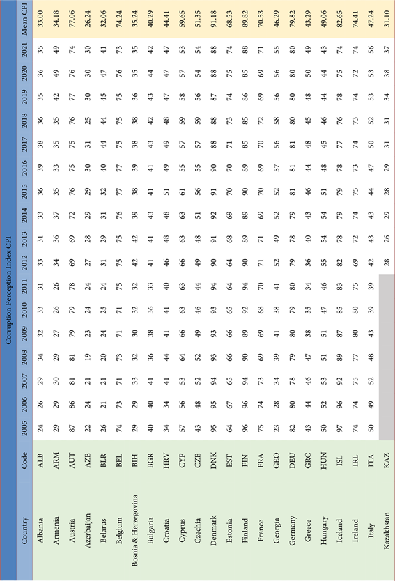
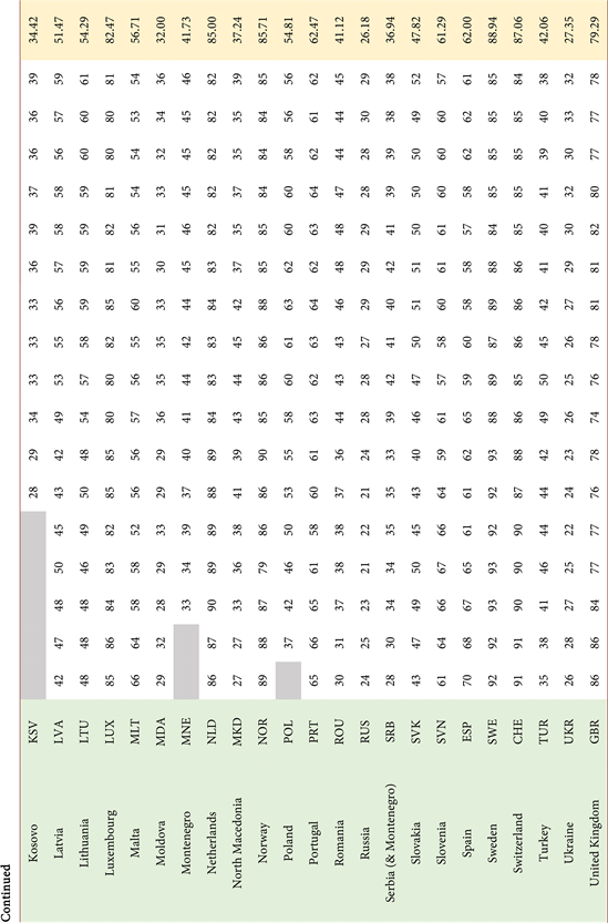
Source: Transparency International (Transparency International, 2021) . : Data Not available. CPI indicators before 2012 have values of [0, 10] scale and were converted to [0, 100] scale in order to obtain compatibility for our analysis.

Appendix 3. GDP Percapita of European Countries

Table A3. GDP per capita of all European Countries for years 2005-2021 (current U.S. $).

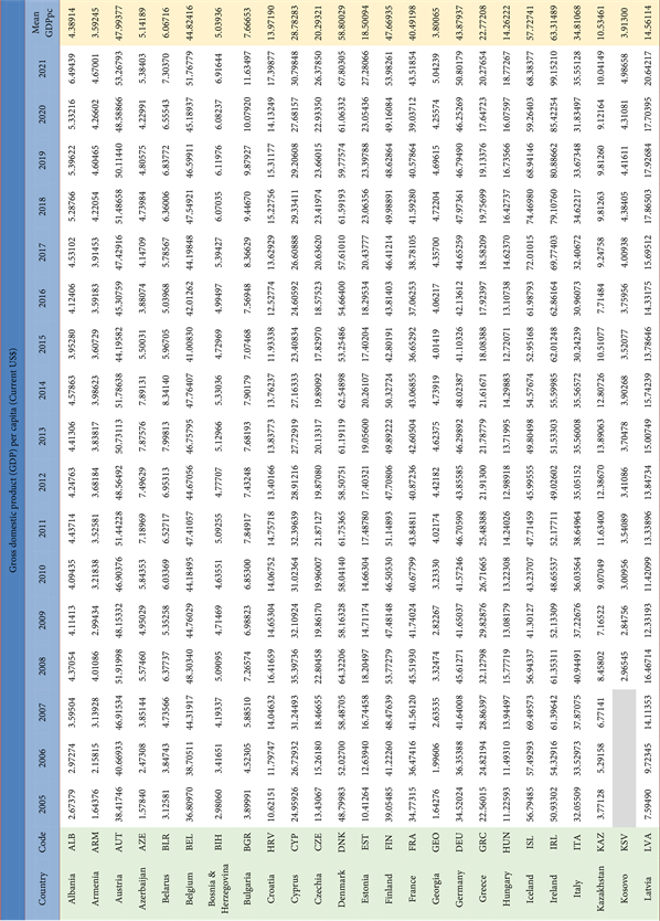
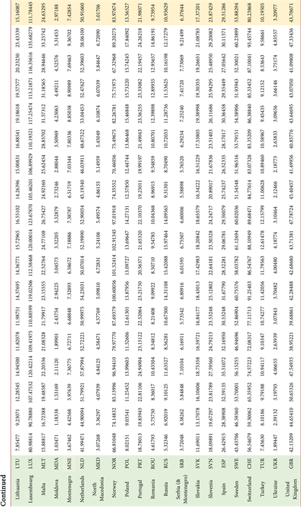
Source: World Bank (2022). : Data Not available. Data Source: World Development Indicators. Source URL: http://data.worldbank.org/indicator/NY.GDP.PCAP.CD (World Bank, 2022b) . Last Updated Date: 16/9/2022. Indicator Code: NY.GDP.PCAP.CD. SOURCE NOTE: GDP per capita is gross domestic product divided by midyear population. GDP is the sum of gross value added by all resident producers in the economy plus any product taxes and minus any subsidies not included in the value of the products. It is calculated without making deductions for depreciation of fabricated assets or for depletion and degradation of natural resources. Data are in current U.S. dollars.

Conflicts of Interest

The authors declare no conflicts of interest regarding the publication of this paper.

References

[1]	Akçay, S. (2002). Corruption and Economic Growth: Across National Study. AfyonKocatepe üniversitesi Iktisadive Idari Bilimler Fakültesi, Working Paper.
[2]	Anastasiou, A., Kalligosfyris, C., & Kalamara, E. (2021) An Analysis of the Efficiency of Tax Administrations of 26 European Countries in 2017. Bulletin for International Taxation, 25, 67-83. https://doi.org/10.59403/1416efw
[3]	Anastasiou, A., Kalligosfyris, C., & Kalamara, E. (2022) Assessing the Effectiveness of Tax Administration in Macroeconomic Stability: Evidence from 26 European Countries. Economic Change and Restructuring, 55, 2237-2261. https://doi.org/10.1007/s10644-022-09384-6
[4]	Anastasiou, A., & Panagiotopoulou, E. (2020) The Strengthening of Economic Growth through the Contribution of Start-Up Entrepreneurship. The Hellenic Open Business Administration Journal, 7, 73-87.
[5]	Barro, R. (1991). Economic Growth in a Cross Section of Countries. The Quarterly Journal of Economics, 106, 407-443. https://doi.org/10.2307/2937943
[6]	Economist Intelligence Unit (2016). Business International. http://www.eiu.com/
[7]	Ehrlich, I., & Lui, F. (1999). Bureaucratic Corruption and Endogenous Economic Growth. Journal of Political Economy, 107, 54-76. https://doi.org/10.1086/250111
[8]	Komninos, D., Dermatis, Z., Anastasiou, A., & Liargovas, P. (2020). The Effect of Over-Taxation and Corruption at Commercial Enterprises in Greece: Evidence from a Survey Experiment. Journal of Statistical and Econometric Methods, 9, 153-170. https://doi.org/10.47260/jsem/vol9410
[9]	Malito, D. V. (2014) Measuring Corruption Indicators and Indices. EUI Working Papers, RSCAS 2014/13. European University, Institute Robert Schuman Centre for Advanced Studies, Global Governance Programme. https://doi.org/10.2139/ssrn.2393335
[10]	Mauro, P. (1995). Corruption and Growth. The Quarterly Journal of Economics, 110, 681-712. https://doi.org/10.2307/2946696
[11]	Mauro, P. (1996). The Effects of Corruption on Growth, Investment, and Government Expenditure. IMF Working Paper, No. 96/98. https://doi.org/10.5089/9781451852097.001
[12]	Mauro, P. (1998). Corruption and the Composition of Government Expenditure. Journal of Public Economics, 69, 263-279. https://doi.org/10.1016/S0047-2727(98)00025-5
[13]	Mocan, N. (2008). What Determines Corruption? International Evidence from Microdata. Economic Inquiry, 46, 493-510. https://doi.org/10.1111/j.1465-7295.2007.00107.x
[14]	Murray, A. (2010). Advances in Location Modeling: GIS Linkages and Contributions. Journal of Geographical Systems, 12, 335-354. https://link.springer.com/article/10.1007/s10109-009-0105-9 https://doi.org/10.1007/s10109-009-0105-9
[15]	Papageorgiou, C., Kalamara, E., Komninos, D., Dermatis, Z., Anastasiou, A., & Liargovas, P. (2018). Corruption Perception Index (CPI), as an Index of Economic Growth for European Countries. Theoretical Economics Letters, 8, 524-537. https://doi.org/10.4236/tel.[phone]
[16]	Podobnik, S., Shao, J., Njavro, D., Ivanov, P. C., and Stanley, H. E. (2008). Influence of Corruption on Economic Growth Rate and Foreign Investment. The European Physical Journal B, 63, 547-550. https://doi.org/10.1140/epjb/e2008-00210-2
[17]	Political Risk Services Inc (2016). International Country Risk Guide. https://www.prsgroup.com/regional-political-risk-index-3/
[18]	Shao, J., Ivanov, P. C., Podobnik, B., & Stanley, H. E. (2007). Quantitative Relations between Corruption and Economic Factors. The European Physical Journal B, 56, 157-166. https://doi.org/10.1140/epjb/e2007-00098-2
[19]	Sritart, Η., & Miyazaki, H. (2022). Geographic Information System (GIS) and Data Visualization. In S. Kanbara, S. Miyagawa, & H. Miyazaki (Eds.), Disaster Nursing, Primary Health Care and Communication in Uncertainty (pp 297-307). Springer. https://link.springer.com/book/10.1007/978-3-030-98297-3 https://doi.org/10.1007/978-3-030-98297-3_26
[20]	The World Bank (2022a). Control of Corruption Index. http://info.worldbank.org/governance/wgi/
[21]	The World Bank (2022b). GPD Per Capita, (Current US$). http://data.worldbank.org/indicator/NY.GDP.PCAP.CD
[22]	Transparency International,(2011). Bribe Payers Index. https://www.transparency.org/en/publications/bribe-payers-index-2011
[23]	Transparency International (2021). Corruption Perception Index 2021. https://www.transparency.org/en/cpi/2021
[24]	Transparency International (2022). Global Corruption Barometer. https://www.transparency.org/en/gcb
[25]	Vlachos, Ι. (2013). Corruption and Economic Growth. Master’s Thesis, University of Peloponnese.