A Comparison of PPO, TD3 and SAC Reinforcement Algorithms for Quadruped Walking Gait Generation

James W. Mock, Suresh S. Muknahallipatna^*

Department of Electrical Engineering and Computer Science, University of Wyoming, Laramie, Wyoming, USA.

DOI: 10.4236/jilsa.2023.151003                

Abstract

Deep reinforcement learning (deep RL) has the potential to replace classic robotic controllers. State-of-the-art Deep Reinforcement algorithms such as Proximal Policy Optimization, Twin Delayed Deep Deterministic Policy Gradient and Soft Actor-Critic Reinforcement Algorithms, to mention a few, have been investigated for training robots to walk. However, conflicting performance results of these algorithms have been reported in the literature. In this work, we present the performance analysis of the above three state-of-the-art Deep Reinforcement algorithms for a constant velocity walking task on a quadruped. The performance is analyzed by simulating the walking task of a quadruped equipped with a range of sensors present on a physical quadruped robot. Simulations of the three algorithms across a range of sensor inputs and with domain randomization are performed. The strengths and weaknesses of each algorithm for the given task are discussed. We also identify a set of sensors that contribute to the best performance of each Deep Reinforcement algorithm.

Keywords

Reinforcement Learning, Machine Learning, Markov Decision Process, Domain Randomization

1. Introduction

Robots have become extremely common within the past few decades. From manufacturing to healthcare, robots play an important integral role in the modern world and with likely be even more integral in the future. However, biomimetic robots, such as humanoid and quadruped robots, are significantly less common. This is primarily due to the limitation of their control algorithms. Many of these controllers utilize sophisticated kinematic and dynamic models separated into submodules so they are easier to manage [1] . These models are difficult and time-consuming to develop and require expertise in both robotics and walking locomotion. Furthermore, these controllers routinely fail to achieve the performance of their biological counterparts. Though more difficult to control, walking robots offer an attractive alternative to typical locomotion systems. Walking robots are more suited for efficiently moving over uneven terrain due to their ability to select where they make contact with the terrain. They also possess an edge with regard to navigation since they are cable of stepping or jumping over obstacles that wheeled or tracked vehicles could not pass [1] [2] .

Despite limited use outside of research applications, many walking robots have been developed. Examples of humanoid robots include NASA’s Valkyrie [3] , Boston Dynamics’ Atlas, and Agility Robotics’ Cassie. Prominent quadruped robots include Boston Dynamics’ Spot, MIT’s Mini Cheetah [4] and Robotic Systems Lab’s ANYmal [5] . All of these robots are sophisticated enough to perform incredible feats of agility but lack the control systems require to operate at their peak performance. To address this shortfall, machine learning (ML) is employed to develop more complex and robust control systems.

Reinforcement learning (RL) is a sub-field of machine learning that learns through interacting with an environment rather than from large datasets as with supervised and unsupervised learning. The goal of RL is to map states to actions with an artificial neural network (ANN) through a trial-and-error process. There are two primary components in RL, the agent and the environment. Figure 1 depicts the agent environment interaction. The agent is responsible for making decisions based on the current state of the environment. The environment is anything the agent cannot change arbitrarily. In robotic applications, it would be natural to assume that the robot is the agent. However, the robot’s actuators, links, sensors, etc. are considered to be part of the environment since the agent cannot explicitly change them. Therefore, the agent is not the robot but actually the control algorithm for the robot.

The fundamental basis for modern reinforcement learning algorithms is the Markov Decision Process (MDP). A MDP is a discrete time state transition model which consists of four components: state space, action space, state transition probabilities and reward. This is usually represented as the tuple ( $\mathcal{S}\mathrm{,}\mathcal{A}\mathrm{,}\mathcal{P}\mathrm{,}\mathcal{R}$ ).

Figure 1. Agent-environment interaction. Image credit: [6] .

The state space is defined by a set of observations of the robot and its environment. An observation at timestep t is given as $s_t\in \mathcal{S}$ . In virtual environments many observations can be obtained directly from the physics engine. For real robots observations usually come in the form of a variety of sensors such as IMUs, motor encoders and cameras. In robotic applications the action space is usually defined by the range of each actuator. The action taken at timestep t is represented as $a_t\in \mathcal{A}$ . $\mathcal{P}$ represents the probability density of the next state $s_{t+1}$ given the current state $s_t$ and action $a_t$ . Reward $r_t\in \mathcal{R}$ is received after transitioning from state $s_t$ to state $s_{t+1}$ , due to action $a_t$ . The reward is always a real scalar value. The function that provides the reward is defined be the system designer to achieve some goal (e.g. walking). The return is defined as the discounted sum of rewards $J_t={\displaystyle {\sum }_{t=0}^T}{\gamma }^t{r}_t$ where $\gamma \in \left(\mathrm{0,1}\right]$ is the discount factor determining the priority of long term rewards. Values of $\gamma$ closer to 0 will cause the agent to prioritize short term rewards over long term rewards.

A solution to an MDP is defined as policy $\pi$ , which maps each state to an action to take in this state to return the highest average reward. RL methods specify how the agent updates its policy as a result of its experience to maximize the return. Additionally, most RL algorithms involve estimating value functions. These functions estimate either the value of being in a particular state or the value of taking particular action. The state-value function, $V_{\pi }\left(s_t\right)$ , for policy $\pi$ is the expected return when starting in $s_t$ and following $\pi$ . $V_{\pi }\left(s_t\right)$ is formally defined as

$V_{\pi }\left(s_t\right)={\mathbb{E}}_{\pi }\left[J_t|s_t\right]={\mathbb{E}}_{\pi }\left[{\displaystyle \underset{k=0}{\overset{\infty }{\sum }}}{\gamma }^k{r}_{t+k+1}|s_t\right].$ (1)

The action-value function, also know as the Q-function, $Q_{\pi }\left(s_t\mathrm{,}{a}_t\right)$ , is the expected return starting from $s_t$ , taking the action $a_t$ , and thereafter following policy $\pi$ . $Q_{\pi }\left(s_t\right)$ is defined as

$Q_{\pi }\left(s_t,a_t\right)={\mathbb{E}}_{\pi }\left[J_t|s_t,a_t\right]={\mathbb{E}}_{\pi }\left[{\displaystyle \underset{k=0}{\overset{\infty }{\sum }}}{\gamma }^k{r}_{t+k+1}|s_t,a_t\right].$ (2)

Both value functions can be estimated from experience. A policy $\pi$ is defined to be better than or equal to a policy ${\pi }^{\prime }$ if its expected return is greater than or equal to that of ${\pi }^{\prime }$ for all states. The optimal policy is defined as the policy with state-value function $V^{\mathrm{<mo>\; *\; </mo>}}\left(s_t\right)=\underset{\pi }{\max }{V}_{\pi }\left(s_t\right)$ and action-value function $Q^{\mathrm{<mo>\; *\; </mo>}}\left(s_t\mathrm{,}{a}_t\right)=\underset{\pi }{\max }{Q}_{\pi }\left(s_t\mathrm{,}{a}_t\right)$ .

Using reinforcement learning over traditional control methods has three potential advantages over traditional controller designs. The first and most significant advantage is the ability to create more sophisticated and robust control algorithms for walking robots. Currently, even mildly rough terrain would pose a serious challenge for most walking robots. The second advantage is a reduction in human effort to develop complex control algorithms. In many cases it may take months or even years to develop control schemes for walking robots. A robot that could learn to walk on its own could drastically reduce the time it takes to develop a suitable control algorithm. The third advantage is the possibility of creating more complex robots. Currently, robots are intentionally simplified so they are easier to control. For example, all of the quadruped robots mentioned previously use the same three degrees of freedom (DOF) per leg configuration. A real dog has at least six DOF per leg excluding toes. This anatomical simplification is likely contributing to the limited capabilities of bio-mimetic robots.

This paper is organized as follows: Section 2 provides a brief summary of the related work. In Section 3, an in-depth mathematical background of the three RL algorithms is presented. Section 4 discusses the experimental setup, training and performance metrics. In Section 5, the simulation results of the training are presented. Section 6 presents the conclusion and future work.

2. Related Work

It has been widely shown that RL algorithms can produce highly sophisticated control policies for tasks in simulations [7] [8] [9] . Three of the top performing algorithms often used for robotics task are Twin Delayed Deep Deterministic Policy Gradient (TD3), Proximal Policy Optimization (PPO) and Soft Actor Critic (SAC). Nevertheless, few performance comparisons of the RL algorithms for robotics applications can be found in the literature, and the few existing comparisons exhibit contradictory performance results. For example, in Fujimoto et al. [9] , TD3 is shown be the top performing algorithm in several robotic walking tasks, including the “HalfCheetah” and “Ant” walking tasks, compared to PPO and SAC. However, this is contradicted in Haarnoja et al. [8] where SAC is shown to be the top performing algorithm for the same tasks compared to TD3 and PPO. Such contradictions make it difficult to ascertain which algorithm is suitable for a particular robot application.

This work seeks to clearly demonstrate how each algorithm performs on a simulated quadruped robotic walking task. Additionally, the algorithms are compared over a variety of sensory inputs. Lastly, each algorithm is tested with domain randomization which is essential for transfer learning of real robots.

3. Overview of Algorithms

RL algorithms are roughly separated into two categories, model-based and model-free. The key distinction between the two is whether or not the agent uses a model of the environment to predict state transitions and rewards. Model-based RL is a deductive approach for solving a problem. The agent uses its understanding of the system to select a best action. Model-based algorithms may learn or be given the environment model. Model-free RL is an inductive approach for solving a problem. The agent uses its past experience to estimate the value of its action. Since model-free algorithm does not rely on the transition probabilities of the MDP in order to find a policy. This is ideal for robots with high dimension, continuous state and action spaces.

The most common type of reinforcement learning used in robotic applications are model-free actor-critic algorithms. Actor-critic methods are time difference (TD) methods that have a separate structures to explicitly represent the policy independent of a value function. The policy structure is known as the actor, because it is used to select actions, and the estimated value function is known as the critic, because it criticizes the actions made by the actor. The critique takes the form of a TD error which is shown in Equation (3).

${\delta }_t=r_t+\gamma V\left(s_{t+1}\right)-V\left(s_t\right)$ (3)

where $r_t$ is the reward at time t given state $s_t$ and action $a_t$ , $\gamma$ is the discount factor and V is the value function implemented by the critic at time t. This scalar signal is the only output of the critic and drives all learning in both actor and critic. Figure 2 shows the actor-critic architecture. Typically, the critic is a state-value function. After each action selection, the critic evaluates the new state to determine whether things have improved or worse than expected. If the TD error is positive, the action is encouraged in the future, whereas if the TD error is negative, it becomes adverse to it.

Model-free actor-critic algorithms can be subdivided into two groups, on-policy and off-policy. On-policy methods, also known as policy optimization, only uses data collected while acting according to the most recent version of the policy to make updates to the policy. Policy optimization also usually involves learning an approximator $V_{\varphi }\left(s_t\right)$ for the on-policy value function $V^{\pi }\left(s_t\right)$ , which is used to update the policy. Q-Learning methods learn an approximator $Q_{\theta }\left(s_t\mathrm{,}{a}_t\right)$ for the optimal action-value function, $Q^{\mathrm{<mo>\; *\; </mo>}}\left(s_t\mathrm{,}{a}_t\right)$ . This optimization is usually performed off-policy. Meaning that each update can use data collected at any point during training, regardless of how the agent was choosing to explore the environment when the data was obtained. These methods often make use of memory buffers that store state-action-state tuples. The primary strength of on-policy methods is that they tend to be stable and reliable. By contrast, off-policy methods tend to be less stable but substantially more sample efficient, because they can reuse data more effectively than on-policy techniques. Both methods have shown good performance in robotic tasks [7] [8] [9] .

Figure 2. Actor-critic architecture. Image credit: [6] .

Three state-of-the-art continuous control policy learning algorithms were chosen to benchmark the gait learning and performance. Proximal Policy Optimization, Twin Delayed Deep Deterministic Policy Gradient and Soft Actor-Critic are consistently shown to be the top performing model-free actor-critic algorithms used for robotic tasks.

PPO is an on-policy RL algorithm that attempts to improve the on Trust Region Policy Optimization (TRPO) algorithm [10] . TRPO attempts to control the policy updates through a Kullback-Leibler (KL) divergence constraint, which quantifies how much a probability distribution differs from another [10] . A major disadvantage of this approach is that it’s computationally expensive. PPO clips the objective function to prevent large updates to the policy [7] . This make PPO easier to implement and computationally faster. The clipped objective function is shown in Equation (4).

$L^{CLIP}\left(\theta \right)={\hat{\mathbb{E}}}_t\left[\min \left(\frac{{\pi }_{\theta }\left(a_t\mathrm{<mo>\; |\; </mo>}{s}_t\right)}{{\pi }_{{\theta }_{old}}\left(a_t\mathrm{<mo>\; |\; </mo>}{s}_t\right)}{\hat{A}}_t\right)\mathrm{,}\text{clip}\left(\frac{{\pi }_{\theta }\left(a_t\mathrm{<mo>\; |\; </mo>}{s}_t\right)}{{\pi }_{{\theta }_{old}}\left(a_t\mathrm{<mo>\; |\; </mo>}{s}_t\right)}\mathrm{,1}-\epsilon \mathrm{,1}+\epsilon \right){\hat{A}}_t)\right]$ (4)

where ${\pi }_{\theta }$ is a stochastic policy. The clipping function limits the lower and upper value of the probability ratio $\frac{{\pi }_{\theta }\left(a_t\mathrm{<mo>\; |\; </mo>}{s}_t\right)}{{\pi }_{{\theta }_{old}}\left(a_t\mathrm{<mo>\; |\; </mo>}{s}_t\right)}$ and $\epsilon$ is the hyperparameter

that sets clip range. The larger the the value of $\epsilon$ , larger the potential policy changes. ${\hat{A}}_t$ is the advantage function shown in Equation (5).

${\hat{A}}_t={\delta }_t+\left(\gamma \lambda \right){\delta }_{t+1}+\cdots +{\left(\gamma \lambda \right)}^{T-t+1}{\delta }_{T-1}$ (5)

where ${\delta }_t$ is the TD error defined in Equation (3), $\gamma$ is the discount factor, and $\lambda$ is the bias-variance trade-off factor for the generalized advantage estimator [11] . During each episode of training the actor collects T timesteps of data. Then the surrogate loss is computed over T timesteps and optimized with minibatch stochastic gradient descent for K epochs. Algorithm 1 summarizes the training process for PPO. As training progresses the policy will try to exploit rewards that it has already found over exploration.

TD3 is an off-policy algorithm that significantly improves upon the deep deterministic policy gradient (DDPG) algorithm [12] . The primary downfall of DDPG is the overestimation bias of the critic network which leads to degraded performance. TD3 implements three key features to improve performance [9] . First, TD3 proposes the use of a clipped double Q-learning algorithm to replace

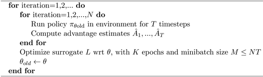
Algorithm 1. PPO, actor-critic style.

the standard Q-learning found in DDPG. The second feature implemented is the use of action noise to reduce overfitting to narrow peaks in the value estimate, a problem often encountered with deterministic policies. The addition of action noise also results in target policy smoothing. For each timestep, both Q networks ( $Q_{{\theta }_1}\mathrm{,}{Q}_{{\theta }_2}$ ) are updated towards the minimum target value of actions selected by the target policy shown in Equation (6)

$y=r_t+\gamma \underset{i=1,2}{\min }{Q}_{{\theta }_{i^{\prime }}}\left(s_{t+1},{\pi }_{{\varphi }^{\prime }}\left(s_{t+1}\right)+\epsilon \right).$ (6)

where $r_t$ is the reward at time t, $\gamma$ is the discount factor and ${\pi }_{\varphi }$ is a deterministic policy, with parameters $\varphi$ , which maximizes the expected return. $\epsilon$ is the clipped Gaussian action noise added and is defined by Equation (7).

$\epsilon ~\text{clip}\left(\mathcal{N}\left(\mathrm{0,}\sigma \right)\mathrm{,}-c\mathrm{,}c\right)$ (7)

The third feature of TD3 is to delay the policy updates by a fixed number of updates to the critic. This is done to suppress the value estimate variance caused by the accumulated TD-error. Parameters $\varphi$ are updated according to the deterministic policy gradient shown in Equation (8).

${\nabla }_{\varphi }J\left(\varphi \right)={\mathbb{E}}_{s_t~p_{\pi }}\left[{{\nabla }_a{Q}_{\pi }\left(s_t\mathrm{,}{a}_t\right)|}_{a_t={\pi }_{\varphi }\left(s_t\right)}{\nabla }_{\varphi }{\pi }_{\varphi }\left(s_t\right)\right]\mathrm{.}$ (8)

where $Q_{\pi }$ is the action-value function defined in Equation (2). TD3 is summarized in Algorithm 2.

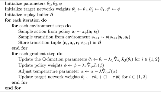
SAC is an off-policy actor-critic algorithm that seeks to maximize a trade-off between expected return and entropy. This encourages a high degree exploration compared to other algorithms. The entropy augmented objective is defined by Equation (9).

${\pi }^{\mathrm{<mo>\; *\; </mo>}}=\underset{\pi }{\arg \max }{\displaystyle \underset{t}{\sum }}{\mathbb{E}}_{\left(s_t\mathrm{,}{a}_t\right)~{\rho }_{\pi }}\left[r_t+\alpha \mathcal{H}\left(\pi \left(\cdot \mathrm{<mo>\; |\; </mo>}{s}_t\right)\right)\right]\mathrm{,}$ (9)

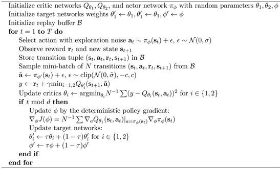
Algorithm 2. TD3.

$r_t$ is the reward at time t and $\alpha$ determines the relative importance of the entropy term, $\mathcal{H}\left(\pi \left(\cdot \mathrm{<mo>\; |\; </mo>}{s}_t\right)\right)=\log \left({\pi }_{\varphi }\left(a_t\mathrm{<mo>\; |\; </mo>}{s}_t\right)\right)$ , against the reward. ${\pi }_{\varphi }$ is a deterministic policy, with parameters $\varphi$ . SAC utilizes two soft Q-functions to mitigate positive bias in the policy improvement step. The soft Q-function parameters, $\theta$ , are trained to minimize the soft Bellman residual given in Equation (10).

$J_Q\left(\theta \right)={\mathbb{E}}_{\left(s_t\mathrm{,}{a}_t\right)~\mathcal{B}}\left[\frac{1}{2}{\left(Q_{\theta }\left(s_t\mathrm{,}{a}_t\right)-\left(r_t+\gamma {\mathbb{E}}_{s_{t+1}~p}\left[V_{\bar{\theta }}\left(s_{t+1}\right)\right]\right)\right)}^2\right]\mathrm{,}$ (10)

where $Q_{\theta }\left(s_t\mathrm{,}{a}_t\right)$ is the minimum of the two soft Q-functions and $\gamma$ is the discount factor. The value function $V_{\theta }$ is the value function implicitly parameterized through the soft Q-function parameters via Equation (11).

$V\left(s_t\right)={\mathbb{E}}_{a_t~\pi }\left[Q\left(s_t\mathrm{,}{a}_t\right)-\alpha \log \pi \left(a_t\mathrm{<mo>\; |\; </mo>}{s}_t\right)\right]$ (11)

The policy parameters are trained by minimizing the objective function in Equation (12).

$J_{\pi }\left(\varphi \right)={\mathbb{E}}_{s_t~\mathcal{B}}\left[{\mathbb{E}}_{a_t~{\pi }_{\varphi }}\left[\alpha \log \left({\pi }_{\varphi }\left(a_t\mathrm{<mo>\; |\; </mo>}{s}_t\right)\right)-Q_{\theta }\left(s_t\mathrm{,}{a}_t\right)\right]\right]\mathrm{.}$ (12)

Additionally, the temperature parameter $\alpha$ can be learned with the following objective function in Equation (13).

$J\left(\alpha \right)={\mathbb{E}}_{a_t~{\pi }_t}\left[-\alpha \log {\pi }_t\left(a_t\mathrm{<mo>\; |\; </mo>}{s}_t\right)-\alpha \bar{\mathcal{H}}\right]$ (13)

The pseudo code for SAC is listed in Algorithm 3. SAC alternates between collecting experience from the environment with the current policy and updating the actor and critic network parameters using stochastic gradients from batches randomly sampled from a replay buffer [8] .

4. Experimental Setup

This section covers the design and setup of the simulated quadruped robot and its environment.

Algorithm 3. SAC.

4.1. System Identification

The simulated environment is constructed using the MuJoCo’s physics simulator. MuJoCo is a free and open source physics engine that aims to facilitate research and development in robotics, biomechanics, graphics and animation [13] . MuJoCo makes it possible to scale up computationally-intensive techniques such optimal control, physically-consistent state estimation, system identification and automated mechanism design, and apply them to complex dynamical systems in contact-rich behaviors. It is well suited for training RL policies for robotic tasks. The simulation environment consists of a single 2 DOF quadruped robot and a ground plane. Figure 3 shows the simulated robot. The robot is similar to the popular Mujoco “Ant” benchmark, but has more realistic actuator torques and includes a variety common sensors that can be found on real robots. These sensors include a body position, body quaternion, foot contact sensors, and actuator position, actuator velocity, actuator load (force), IMUs on the body and legs. The large yellow spheres at the end of the feet represent the feet contact sensors. The smaller yellow spheres on the legs represent the locations of the IMU sensors. An additional IMU is located at the center of the main body. The body position and quaternion are measured at the center of the main body. Gaussian noise was added to each sensor to imitate the imprecision of real sensors. The robot has eight actuators. No actuator or latency models were considered for the simulation.

4.2. State and Action Spaces

Actions $a_t$ are actuator target positions mapped to values between −1 and 1. The state $s_t$ consists of the most recent readings of various sensors. Seven sensor configurations were tested with each algorithm to identify the best possible level of sensory input for each algorithm. The sensors used in each configuration are listed in Table 1. The first configuration (v0) uses only the body quaternion for the state space and the last configuration (v6) utilizes all sensor data on the robot for the state space.

Figure 3. Simulated quadruped robot testbed.

Table 1. State space configurations.

4.3. Reward Function

The reward function was designed to encourage a stable forward walking gait at a target velocity ${\hat{v}}_x$ with a target orientation $\hat{q}$ . The reward function is given by the Equation (14)

$\begin{array}{c}R=r_H+w_A\ast {\displaystyle \sum }{\left(a_t\right)}^2+w_V\ast {\displaystyle \sum }{\left({\Omega }_t\right)}^2+w_{TV}\ast \left|{\hat{v}}_x-v_x\right|+w_D\ast \left|v_y\right|\\ +w_{TQ}\ast \text{sum}\left(\left|\hat{q}-q\right|\right),\end{array}$ (14)

where $r_H$ is the reward for not experiencing a catastrophic failure, such as flipping over. $w_A$ is the weight that determines the importance of penalizing actions, $a_t$ . $w_V$ is the weight that determines the importance of penalizing actuator velocities, ${\Omega }_t$ . $w_{TV}$ is the importance weight for the target velocity and $w_D$ is the importance weight for penalizing linear velocity in the lateral direction. $w_{TQ}$ is the importance weight for deviation from the target quaternion. The final weights used are listed in Table 2.

4.4. Domain Randomization

The inevitable imperfections of physics simulations will automatically be exploited by any optimization method to achieve an improvement. However, since these exploits don’t exist in the real world, policies transferred to the real world will not perform as expected. This is known as the simulation optimization bias (SOB) [14] . One method to combat SOB is to randomize parameters of the simulation. Unlike system identification which aims to carefully model the real world, domain randomization aims to randomize the visuals or system dynamics of a simulation to encourage generalization. System identification and domain randomization are often used together to achieve better results [1] [15] [16] . Early domain randomization techniques largely consisted of adding i.i.d. noise to observations and actions [14] . Newer techniques involve changing the appearance and core dynamics of a simulated environment. Vision based learning have a particularly wide reality gap because it is very difficult to generate sufficiently high-quality rendered images [16] . Additionally, simulated cameras fail to incorporate noise and optical distortions produced by real cameras [17] . For a vision based object manipulation tasks, Pinto et al. [18] randomized textures,

Table 2. Reward function parameters.

lighting and the position of the camera. They found that policies trained without domain randomization failed to perform when transferred to the real robot. For non-vision based robots parameters like mass, friction coefficients and actuator behavior are randomized. Tan et al. [15] found that using inertia randomization when learning a quadruped gait significantly improves robustness at the cost optimality. Meaning that using domain randomization causes the simulated policy to have degraded performance but will perform better on the physical robot. Adversarial disturbances to the agent are another common form of domain randomization. Rudin et al. [19] implemented this idea by pushing the simulated robot every 10 seconds. The robots’ base is accelerated up to ±1 m/s in both x and y directions. This results in a highly stable and dynamic walking gait which was successfully deployed on a real robot.

4.5. Training

The simulated environment is setup to recreate the agent-environment described previously. Every 50 ms in simulation time the agent reads in the current state of the robot which is described by the robot’s sensors. The sensors that are used depend on which configuration is being tested. The agent then uses the state space to generate target motor positions. The updated motor positions are sent the robot. After 50 ms the state of the robot is read again and a reward is given based on the reward function described in Section 4.3. This process repeats for one thousand iterations. Upon completion of an episode of one thousand steps the simulation is reset. TD3 and SAC make updates following the end each episode while PPO makes updates at a fixed interval. Each algorithm was trained on each sensor configuration for three million steps. This was repeated five times for each algorithm configuration combination.

To evaluate if an algorithm is suitable for transfer learning to a real robot a second group of policies were trained under identical circumstances except with domain randomization. The group using dynamics randomization experienced random variations in robot’s mass, inertia and friction coefficients as well as variations in actuator stiffness, friction loss, damping, and reflected inertia.

4.6. Models and Hyperparameters

To compare optimal performance of each algorithm the Stable-Baselines3 (SB3) implementation was used for all three algorithms. SB3 is a set of reliable implementations of reinforcement learning algorithms in PyTorch [20] . Several combinations of hyperparameters were tested for each algorithm. However, the default SB3 values were found to be the best. Table 3 summarizes the ANN architectures and hyperparameters used for each algorithm.

Table 3. Hyperparameters for each RL algorithm.

4.7. Performance Metrics

The performance of trained policies was evaluated by comparing the quantitative metrics of walking gait for the three algorithms. The metrics associated with the walking gait are the average forward velocity (m/s), average forward velocity variance, average lateral velocity (m/s), average lateral velocity variance, and quaternion root mean square deviation (RMSD). Ideally an agent should achieve an average forward velocity of 0.5 m/s, a lateral velocity of 0.0 m/s, no forward or lateral velocity variance and no deviation in the quaternion. The maximum reward per time step that can be achieved is 1.0. Performance was evaluated as the average of all five trials over one thousand steps or fifty seconds in simulation time.

5. Results

This section provides an analysis of the simulated agent’s performance. It also offers a comparison of algorithm performance across sensor configurations and with domain randomization.

5.1. Training without Domain Randomization

Figures 4-6 show the average learning curve in terms of the reward of each robot configuration using PPO, TD3 and SAC respectively without domain randomization. Across all three algorithms configurations v2, v3, and v4 achieve the

Figure 4. Average learning curve for each sensor configuration using PPO algorithm.

Figure 5. Average learning curve for each sensor configuration using TD3 algorithm.

Figure 6. Average learning curve for each sensor configuration using SAC algorithm.

highest average reward. Configuration v2 is the first sensor configuration that includes actuator velocities. Unlike the body quaternion and actuator position, actuator velocity has a temporal relation which is likely the reason its inclusion in the state space significantly improves learning performance. The addition of actuator load in configuration v3 and contact sensors in configuration v4 do not improve the max reward beyond configuration v2. The addition of more sensors does not degrade learning till the IMU sensor data is added in configurations v4 and v5. SAC was the only algorithm to achieve a high reward for these configurations. However, training is significantly slower compared to other configurations. Configuration v6 achieve a reward comparable to configurations v2, v3, and v4 while configuration v5 has a slightly lower max reward. The fact that configuration v6 is higher than v5 would indicate that the policy is developing a form of sensor fusion for the IMU data. The inclusion of IMU data significantly increases the size of the state space. This indicates that for agents with large state spaces SAC may perform better. In contrast, PPO was the only algorithm to achieve an average reward higher than 500 using configurations v0 and v1, though they are still not on par with configurations v2, v3 and v4. This indicates that PPO performs better with smaller state spaces. It can also be seen that the TD3 and SAC agents have significantly steeper learning curves compared to PPO agents. This is due to the fact that off-policy algorithms make far more updates than on-policy algorithms. However, from Figure 5 it can be seen that TD3 takes significantly longer to reach its max reward compared to the other two algorithms. PPO and SAC converge at their maximum reward before five hundred thousand steps, TD3 takes nearly two million steps to converge.

Tables 4-6 show the average quantitative metrics of the walking gaits achieved for each sensor configuration. Table 4 shows the average performance of each sensor configuration using PPO. Configurations v2, v3 and v4 show the best performance with average forward velocities very close to the target velocity of 0.5 m/s. Additionally, all other metrics are close to zero as desired. Overall, it appears that configuration v3 performs the best as it was able to achieve an average velocity closest to the target velocity. Configurations v0 and v1 also seem

Table 4. Average performance of each sensor configuration trained with PPO algorithm.

Table 5. Average performance of each sensor configuration trained with TD3 algorithm.

Table 6. Average performance of each sensor configuration trained with SAC algorithm.

to generate stable walking gaits. However, they were unable to come as close to the target velocity as the previously mentioned configurations. Lastly, configurations v5 and v6 fail to generate any walking gaits.

From Table 5, it can be seen that the TD3 algorithm only generates walking gaits for configurations v1 through v4. Like PPO, the average forward velocity for configuration v1 does not reach the target velocity. Also similar to PPO, the best gait was achieved with configuration v3. For configurations v2, v3, and v4 TD3 achieves a higher average velocity than both PPO and SAC. However, the other four metrics seem to be worse as a result. For configurations v5 and v6 all agents learn to remain still to achieve a maximum reward.

Table 6 shows that SAC was able to generate walking gaits for all configurations except v0. Like PPO and TD3, the average velocity of configuration v1 fails to achieve to desired velocity. Configurations v4 and v6 are the top performing configurations in terms of average forward velocity.

5.2. Training with Domain Randomization

Figures 7-9 show the average learning curve in terms of the reward of each robot configuration using PPO, TD3 and SAC respectively using domain

Figure 7. Average learning curve for each sensor configuration using PPO algorithm with domain randomization.

Figure 8. Average learning curve for each sensor configuration using TD3 algorithm with domain randomization.

Figure 9. Average learning curve for each sensor configuration using SAC algorithm with domain randomization.

randomization. The learning curves are very similar to the simulations without domain randomization. The most significant difference being the lower maximum reward compared to agents trained without domain randomization. This is expected since randomization of dynamics makes walking much more difficult with the goal of achieving a more robust walking gait. Additionally, for some algorithm-configuration combinations, training is significantly slower. All configurations of PPO require approximately an additional three hundred thousand steps to reach their maximum reward. TD3 shows a notable preference for configuration v4 over v2 and v3 in terms of learning speed. Likewise, SAC also shows a slight preference for configuration v4. This indicates that foot sensors should be an important sensory input for real-world walking tasks.

Tables 7-9 show the average performance metrics for each algorithm-configuration combination. A notable difference that can be observed is the overshooting of the target forward velocity for PPO and TD3. TD3 especially overshoots be a considerable margin for configurations v2 and v3. Interestingly, SAC does not demonstrate the same overshooting behavior. It can also be seen that

Table 7. Average performance of each sensor configuration trained with PPO algorithm and domain randomization.

Table 8. Average performance of each sensor configuration trained with TD3 algorithm and domain randomization.

Table 9. Average performance of each sensor configuration trained with SAC algorithm and domain randomization.

the performance of configuration v0 with PPO is significantly worse than without domain randomization. This can also be seen with configuration v1 with TD3. Lastly, SAC shows a significant performance increase for configurations v5 and v6 over other configurations.

5.3. Results Summary

• Actuator velocity is essential for generating stable walking gaits for all three RL algorithms.

• The performance of all three algorithms is very similar for configurations v2, v3 and v4 both with and without domain randomization.

• TD3 and SAC both learn significantly quicker than PPO.

• PPO excels with minimal state spaces but performs very poorly with the addition of IMU data.

• SAC was the only algorithm to generate a stable walking gait with IMU data both with and without domain randomization.

• TD3 does not perform well with minimal state spaces or with the addition of IMU data.

• Domain randomization does affect the performance of all three algorithms in a negative manner. However, in most cases the algorithms are still able to generate stable gaits comparable to policies trained without domain randomization.

• Contact sensors in the feet significantly improve performance in all three algorithms when using domain randomization.

6. Conclusion

In this paper, the performance of three state-of-the-art RL algorithms was compared with the walking gait of a quadruped robot. The performance of the three algorithms was studied on a quadruped robot simulated by modeling the robot using the MuJoCo’s native MJCF modeling language. Each algorithm performance was evaluated in seven different state spaces along with addressing the simulation optimization basis (domain randomization). The performance results demonstrated that the performance of the three algorithms was dependent on the sensor configurations, i.e., the state space. Without domain randomization, the SAC algorithm was able to generate walking gaits for all state spaces other than the state space which consisted only of the body quaternion. The PPO and TD3 algorithms were not able to generate walking gaits for the state spaces including the accelerometer and gyro data. The TD3 and PPO algorithms were noticed to have overshooting of the target velocity with domain randomization while SAC did not exhibit overshooting. Also, SAC had a significant performance improvement with the use of an accelerometer and gyro along with domain randomization. The performance results of the three algorithms do not present a clear winner. The results demonstrate the preference of the algorithms to state spaces. It can be seen that PPO tends to perform better with smaller state spaces while SAC excels with larger state spaces. Finally, it was shown that domain randomization does not significantly degrade policy performance in most cases for any algorithm. Even though all three algorithms can potentially be used for transfer learning on real robots, their performance needs to be evaluated on a real physical quadruped robot.

Conflicts of Interest

The authors declare no conflicts of interest regarding the publication of this paper.

References

[1]	Hwangbo, J., Lee, J., Dosovitskiy, A., Bellicoso, D., Tsounis, V., Koltun, V. and Hutter, M. (2019) Learning Agile and Dynamic Motor Skills for Legged Robots. Science Robotics, 4. http://arxiv.org/abs/1901.08652 https://doi.org/10.1126/scirobotics.aau5872
[2]	Biswal, P. and Mohanty, P.K. (2021) Development of Quadruped Walking Robots: A review. Ain Shams Engineering Journal, 12, 2017-2031. https://doi.org/10.1016/j.asej.2020.11.005 https://www.sciencedirect.com/science/article/pii/S2090447920302501
[3]	Radford, N.A., Strawser, P., Hambuchen, K., Mehling, J.S., Verdeyen, W.K., Donnan, A.S., Holley, J., Sanchez, J., Nguyen, V., Bridgwater, L., Berka, R., Ambrose, R., Myles Markee, M., Fraser-Chanpong, N.J., McQuin, C., Yamokoski, J.D., Hart, S., Guo, R., Parsons, A., Wightman, B., Dinh, P., Ames, B., Blakely, C., Edmondson, C., Sommers, B., Rea, R., Tobler, C., Bibby, H., Howard, B., Niu, L., Lee, A., Conover, M., Truong, L., Reed, R., Chesney, D., Platt Jr., R., Johnson, G., Fok, C.-L., Paine, N., Sentis, L., Cousineau, E., Sinnet, R., Lack, J., Powell, M., Morris, B., Ames, A. and Akinyode, J. (2015) Valkyrie: Nasa’s First Bipedal Humanoid Robot. Journal of Field Robotics, 32, 397-419. https://doi.org/10.1002/rob.21560 https://onlinelibrary.wiley.com/doi/abs/10.1002/rob.21560
[4]	Bledt, G., Powell, M.J., Katz, B., Carlo, J.D., Wensing, P.M. and Kim, S. (2018) MIT Cheetah 3: Design and Control of a Robust, Dynamic Quadruped Robot. 2018 IEEE/RSJ International Conference on Intelligent Robots and Systems, Madrid, 1-5 October 2018, 2245-2252. https://doi.org/10.1109/IROS.2018.8593885
[5]	Hutter, M., Gehring, C., Jud, D., Lauber, A., Bellicoso, C. D., Tsounis, V., Hwangbo, J., Bodie, K., Fankhauser, P., Bloesch, M., Diethelm, R., Bachmann, S., Melzer, A. and Hoepflinger, M. A. (2016) ANYmal—A Highly Mobile and Dynamic Quadrupedal Robot. 2016 IEEE/RSJ International Conference on Intelligent Robots and Systems, Daejeon, 9-14 October 2016, 38-44. https://doi.org/10.1109/IROS.2016.7758092
[6]	Sutton, R.S. and Barto, A.G. (2018) Reinforcement Learning: An Introduction. 2nd Edition, The MIT Press, Cambridge. http://incompleteideas.net/book/the-book-2nd.html
[7]	Schulman, J., Wolski, F., Dhariwal, P., Radford, A. and Klimov, O. (2017) Proximal Policy Optimization Algorithms. ArXiv: 1707.06347. http://arxiv.org/abs/1707.06347
[8]	Haarnoja, T., Zhou, A., Abbeel, P. and Levine, S. (2018) Soft Actor-Critic: Off-Policy Maximum Entropy Deep Reinforcement Learning with a Stochastic Actor. ArXiv: 1801.01290. http://arxiv.org/abs/1801.01290
[9]	Fujimoto, S., van Hoof, H. and Meger, D. (2018) Addressing Function Approximation Error in Actor-Critic Methods. ArXiv: 1802.09477. http://arxiv.org/abs/1802.09477
[10]	Schulman, J., Levine, S., Moritz, P., Jordan, M.I. and Abbeel, P. (2015) Trust Region Policy Optimization. ArXiv: 1502.05477. http://arxiv.org/abs/1502.05477
[11]	Schulman, J., Moritz, P., Levine, S., Jordan, M.I. and Abbeel, P. (2016) High-Dimensional Continuous Control Using Generalized Advantage Estimation. 4th International Conference on Learning Representations, ICLR 2016, San Juan, 2-4 May 2016. http://arxiv.org/abs/1506.02438
[12]	Lillicrap, T. P., Hunt, J. J., Pritzel, A., Heess, N., Erez, T., Tassa, Y., Silver, D. and Wierstra, D. (2016) Continuous Control with Deep Reinforcement Learning. 4th International Conference on Learning Representations, ICLR 2016, San Juan, Puerto Rico, 2-4 May 2016. http://arxiv.org/abs/1509.02971
[13]	Todorov, E., Erez, T. and Tassa, Y. (2012) Mujoco: A Physics Engine for Model-Based Control. 2012 IEEE/RSJ International Conference on Intelligent Robots and Systems, Vilamoura-Algarve, 7-12 October 2012, 5026-5033. https://doi.org/10.1109/IROS.2012.6386109
[14]	Muratore, F., Gienger, M. and Peters, J. (2021) Assessing Transferability from Simulation to Reality for Reinforcement Learning. IEEE Transactions on Pattern Analysis and Machine Intelligence, 43, 1172-1183. http://arxiv.org/abs/1907.04685 https://doi.org/10.1109/TPAMI.2019.2952353
[15]	Tan, J., Zhang, T., Coumans, E., Iscen, A., Bai, Y., Hafner, D., Bohez, S. and Vanhoucke, V. (2018) Sim-to-Real: Learning Agile Locomotion for Quadruped Robots. ArXiv: 1804.10332. http://arxiv.org/abs/1804.10332 https://doi.org/10.15607/RSS.2018.XIV.010
[16]	Zhao, W., Queralta, J.P. and Westerlund, T. (2020) Sim-to-Real Transfer in Deep Reinforcement Learning for Robotics: A Survey. 2020 IEEE Symposium Series on Computational Intelligence, Canberra, 1-4 December 2020, 737-744. https://arxiv.org/abs/2009.13303 https://doi.org/10.1109/SSCI47803.2020.9308468
[17]	Tobin, J., Fong, R., Ray, A., Schneider, J., Zaremba, W. and Abbeel, P. (2017) Domain Randomization for Transferring Deep Neural Networks from Simulation to the Real World. 2017 IEEE/RSJ International Conference on Intelligent Robots and Systems, Vancouver, 24-28 September 2017, 23-30. http://arxiv.org/abs/1703.06907 https://doi.org/10.1109/IROS.2017.8202133
[18]	Pinto, L., Andrychowicz, M., Welinder, P., Zaremba, W. and Abbeel, P. (2017) Asymmetric Actor Critic for Image-Based Robot Learning. ArXiv: 1710.06542. http://arxiv.org/abs/1710.06542 https://doi.org/10.15607/RSS.2018.XIV.008
[19]	Rudin, N., Hoeller, D., Reist, P. and Hutter, M. (2021) Learning to Walk in Minutes Using Massively Parallel Deep Reinforcement Learning. ArXiv: 2109.11978. https://arxiv.org/abs/2109.11978
[20]	Raffin, A., Hill, A., Gleave, A., Kanervisto, A., Ernestus, M. and Dormann, N. (2021) Stable-Baselines3: Reliable Reinforcement Learning Implementations. Journal of Machine Learning Research, 22, 1-8. http://jmlr.org/papers/v22/20-1364.html