Population Interaction Dynamics Analysis of an Algae-Fish System

Ziyou Zhuang¹, Jueyuan Yan¹, Xinyu Xie¹, Lihua Dai¹, Chaoyue Huang¹, Fangfang Chen¹, Hengguo Yu^1,2*

¹School of Mathematics and Physics, Wenzhou University, Wenzhou, China.
²Key Laboratory for Subtropical Oceans & Lakes Environment and Biological Resources Utilization Technology of Zhejiang, Wenzhou University, Wenzhou, China.

DOI: 10.4236/am.2022.136035                

Abstract

In this paper, before the implementation of ecological laboratory experiments, the population interaction dynamics of an algae-fish system were studied mathematically and numerically. The purpose of this study was to explore how filter-feeding fish population affects the growth dynamics of the algae population. Mathematically theoretical works have been pursuing the investigation of some key conditions for stability of the equilibrium and existence of Hopf bifurcation. Numerical simulation works have been parsing the discovery of the growth dynamics of the algae population in view of population interaction dynamics, which in turn could prove the feasibility of the theoretical derivation and reveal the relationship between filter-feeding fish abundance and algal biomass in fish-drift algae communiyua. Furthermore, it was successful to show that the filter-feeding fish population may be a crucial factor in controlling the proliferation of the algae population, which could also directly grasp the evolution of community dynamics. All these results were expected to be useful in the study of community dynamics and laboratory elimination experiment of the algae population.

Keywords

Algae Population, Filter-Feeding Fish, Population Interaction Dynamics, Hopf Bifurcation, Stability

1. Introduction

Eutrophication of lake and reservoir has been widely and intensively investigated for decades, which also has been regarded as the concentration of natural evolution process caused by the influence of human social activities [1]. The essence of eutrophication was that the input and output of nutrients were out of balance, which could lead to the imbalance of species distribution in water ecosystem and the rapid growth of single species, and then the flow of material and energy in the system was destroyed, which could make the whole water ecosystem gradually perish [2]. Algal bloom was the result of eutrophication and specific conditions, which could seriously affect the water environment, human health and environmentally sustainable development [3].

Fish species have always used an effective measure to control algal bloom because fishes could eat and digest some algae populations, which have been widely applied in controlling harmful algal blooms in the lake ecosystem [4]. Many scholars have tried to reduce or inhibit algal blooms using filter-feeding fish, such as silver carp and bighead carp, which have been shown to be effective in controlling algal blooms in China and other countries. Xie and Liu [5] have investigated how to control cyanobacteria blooms using filter-feeding fish, they believed that an increased stocking of the lake with carp played a decisive role in the elimination of cyanobacteria blooms and both silver and bighead carp could eliminate cyanobacteria blooms directly by grazing, these results were significant for biotic control of harmful algal blooms. Starling [6] has conducted a mesocosm experiment to assess the impact of moderate silver carp (Hypophthalmichthysmolitrix) biomass on the plankton community and water quality of eutrophic Parano Reservoir (Brasilia, Brazil), the results suggested that stocking silver carp in Parano Reservoir to control blue-green algae was a promising biomanipulation practice, but this result was very meaningful. Kulczycki et al. [7] have indicated that significant relationships exist between the abundances of both the fish (code goby Gobiosoma robustum) and drift algae biomass, but it was still of interest. Judit et al. [8] have implied that the presence of these filter-feeding fish (asian carps and bighead carp) could alter the phytoplankton species composition and promote the dominance of taxa that are able to resist digestion. Shen et al. [9] have experimentally studied the effect of combining two native filter feeders, bighead carp (Aristichthysnobilis) and Asian clam (Corbiculafluminea), to control nuisance cyanobacterial blooms, they suggested that the combination of filter-feeding fish and clams may enhance water clarity and it may therefore potentially be a useful restoration tool, and these results have played an important role in the control of algal blooms. Based on the above analysis, it was worth affirming that the filter-feeding fish could control or inhibit algal blooms.

Population interaction dynamics was the dynamic relationship between population and population, which can regulate and control the evolution process and development trend of population, such as Hopf bifurcation and stability, which referred to the dynamic switching between the stable equilibrium point (Population biomass tends to be a quantitative one) and the stable limit cycle (Population biomass oscillates between two constant values). Deka et al. [10] have investigated stability and Hopf bifurcation in a two-prey and one-predator system, they observed that intra-specific interference factor was an important parameter in governing stability and Hopf bifurcation, which has certain novelty. Liu et al. [11] have studied Hopf bifurcation of a diffusive predator-prey model, they found that the diffusion and delay could induce spatially bifurcating period solution, the result was good. Datta et al. [12] have inquired into bifurcation and bio-economic of a prey-generalist predator model with nonlinear age-selective prey harvesting, they suggested that the age-selective prey harvesting system could go a Hopf bifurcation with respect to the maturation delay, the research ideas were innovative. Wei [13] has found that prey switching may stabilize the population dynamics and has a synergistic effect on enhancing coexistence and stabilizing population dynamics under predator interference, these results were excellent. Ivanov and Dimitrova [14] have looked into global stability of a predator-prey model with generic birth and death rates for predator. Hajnová and Pribylová [15] have dissected bifurcation manifolds in predator-prey models, their method provided formulas for bifurcation manifolds in commonly studied cases in applied research for the fold, transcritical, cusp, Hopf and Bogdanov-Takens bifurcation, these research results were also excellent. Gao et al. [16] have parsed bifurcation in a diffusive ratio-dependent predator-prey model with predator harvesting, they derived some condition for determining the direction of Hopf bifurcation and the stability of the bifurcating periodic solution, its content was relatively new. Lv et al. [17] have discussed bifurcations and simulations of two predator-prey model with nonlinear harvesting, they proclaimed that nonlinear harvesting could make the dynamics of the model more complicated, including bistability, transcritical bifurcation and Hopf bifurcation, these results were quite important. Bulai and Venturino [18] have pointed out that the stable solution was independent of the shape of the herb for competition, its influence was immeasurable. Sahoo and Poria [19] have proposed that the predator-prey system with fading memory has rich dynamic behaviors, such as supercritical and subcritical Hopf bifurcation, these results were still important. Pal et al. [20] have raised that an increase in the hunting cooperation induced fear may destabilize the system and produce periodic solution via Hopf bifurcation and limit cycles may be supercritical and subcritical, these results were crucial. Falconi et al. [21] have characterized the existence of Hopf bifurcation and proved that this model exhibited either one, two or three small amplitude periodic solution, these results were quite subtle. In conclusion, as far as we know, these authors have made some important results in population interaction dynamics, which can greatly promoted the development of ecological population dynamics.

Based on the above analysis, we can see that the filter-feeding fish have been thought to be suited to control algal blooms directly in the subtropical lake reservoir, some similar research results can be seen in the paper [22] [23] [24] [25]. Taking it as an incentive, the main aim of the paper is to inquire into the relationship between filter-feeding fish abundance and algal biomass with the help of mathematical ecological model and explore filter-feeding fish population how to affect the growth dynamics of the algae population by means of population interaction dynamics, which can support a theoretical basis for the algal-fish ecological control experiment and provide a different insight to understand the ecological control mechanism of algal blooms.

2. Biological Modeling

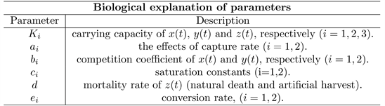
Based on the physical and biological processes in the aquatic ecosystem, with the help of differential ecological modeling theory, some modeling assumptions were given as follows:

1) The laboratory experiment of the interaction dynamics between algae population and filter-feeding fish population is a closed water ecosystem, species concentration is always evenly distributed in space and changed instantaneously with time, $x\left(t\right)$, $y\left(t\right)$ and $z\left(t\right)$ represent respectively the density of cyanobacteria, green algae and filter-feeding fish.

2) The filter-feeding fish z will feed on algae population and zooplankton, which suggests that the growth of filter-feeding fish mainly depends on the abundance of algae and zooplankton, the function of zooplankton affecting the abundance of filter-feeding fish is $r_{3}z\left(1-\frac{z}{K_3}\right)$ with intrinsic growth rate $r_3$.

3) The algae population includes cyanobacteria x and green algae y, the cyanobacteria and green algae have a competitive relationship, the competitiveness of cyanobacteria is greater than that of green algae in the same water area ( $b_1>b_2$ ).

4) The growth kinetics of cyanobacteria x and green algae y are logistic manner $r_{1}x\left(1-\frac{x}{K_1}\right)$ and $r_{2}y\left(1-\frac{y}{K_2}\right)$ with intrinsic growth rate $r_1$ and $r_2$.

5) According to the competition between populations and within populations, it can been assumed that competition among populations is less than that within populations, thus

$b_1<\frac{r_1}{K_2},b_2<\frac{r_2}{K_1}.$ (2.1)

6) In view of the previous algae growth simulation experiments, in order to maintain the operability of simulation test and the recyclability of aquatic ecosystem, the sum of the maximum regeneration biomass must be greater than the minimum regeneration critical threshold 4 (the routine basic data of laboratory simulation test). Thus, we will assume that the key parameters of population growth can satisfy the following conditions:

$r_1{K}_1{e}_1+r_2{K}_2{e}_2+r_3{K}_3>4.$ (2.2)

Based on the above assumptions and modelling is playing an increasing role in helping to investigate the relationship between filter-feeding fish abundance and algal biomass, the paper will consider an algae-fish ecological model, which can be described by the following differential equations:

$(\begin{array}{l}\frac{\text{d}x}{\text{d}t}=r_{1}x\left(1-\frac{x}{K_1}\right)-b_{1}xy-\frac{a_{1}xz}{c_1+x}=x{f}_{\left(1\right)}\left(x,y,z\right),\\ \frac{\text{d}y}{\text{d}t}=r_{2}y\left(1-\frac{y}{K_2}\right)-b_{2}xy-\frac{a_{2}yz}{c_2+y}=y{f}_{\left(2\right)}\left(x,y,z\right),\\ \frac{\text{d}z}{\text{d}t}=\frac{e_1{a}_{1}xz}{c_1+x}+\frac{e_2{a}_{2}yz}{c_2+y}-dz+r_{3}z\left(1-\frac{z}{K_3}\right)=z{f}_{\left(3\right)}\left(x,y,z\right),\end{array}$ (2.3)

with the initial conditions:

$x\left(0\right)=x_0>0,\mathrm{<mtext>\; \hspace{0.17em}\; </mtext>}y\left(0\right)=y_0>0,\mathrm{<mtext>\; \hspace{0.17em}\; </mtext>}z\left(0\right)=z_0>0.$ (2.4)

Here

$\begin{array}{l}{f}_{\left(1\right)}\left(x,y,z\right)=r_1\left(1-\frac{x}{K_1}\right)-b_{1}y-\frac{a_{1}z}{c_1+x},\\ f_{\left(2\right)}\left(x,y,z\right)=r_2\left(1-\frac{y}{K_2}\right)-b_{2}x-\frac{a_{2}z}{c_2+y},\\ f_{\left(3\right)}\left(x,y,z\right)=\frac{e_1{a}_{1}x}{c_1+x}+\frac{e_2{a}_{2}y}{c_2+y}-d+r_3\left(1-\frac{z}{K_3}\right).\end{array}$

and

3. Mathematical Analysis

As we all know, the essence of algal bloom outbreak is the essential change of the internal operation state of the water ecosystem, in which the critical threshold phenomenon is particularly obvious. And, the critical threshold phenomenon can refer to the situation that a process suddenly can enter another state when the influence factors or environmental conditions reach a certain degree (threshold), its essence is a process from quantitative change to qualitative change, from one state to another completely different state. Hence, we will explore critical threshold phenomena based on mathematical analysis and dynamic behaviors.

Lemma 3.1 [26]. If $a,b>0$ and $\frac{\text{d}x\left(t\right)}{\text{d}t}\le (\ge )x\left(t\right)\left[a-bx\left(t\right)\right]$ with $x\left(0\right)>0$, then ${\lim }_{t\to +\infty }\sup x\left(t\right)\le \frac{a}{b}$ ( ${\lim }_{t\to +\infty }\inf x\left(t\right)\ge \frac{a}{b}$ ).

In fact, the above lemma is quantitatively equivalent to the following lemma.

Lemma 3.2 [27]. If $a,b>0$ and $\frac{\text{d}x\left(t\right)}{\text{d}t}\le x\left(t\right)\left[a-bx\left(t\right)\right]$ with $x\left(0\right)>0$, then for all $t\ge 0$, $x\left(t\right)\le \frac{a}{b-c{\text{e}}^{-at}}$, with $c=b-\frac{a}{x\left(0\right)}$. In particular, $x\left(t\right)\le \max \left\{x\left(0\right),\frac{a}{b}\right\}$, for all $t\ge 0$.

Now, we prove the positivity and boundedness of solutions as well as the permanence of the system (2.3).

3.1. Positivity and Boundedness of Solutions

Proposition 3.1. 1) All solutions $\left(x\left(t\right)\mathrm{,}y\left(t\right)\mathrm{,}z\left(t\right)\right)$ of the system (2.3) with the initial conditions (2.4) are positive for all $t\ge 0$.

2) All solutions $\left(x\left(t\right)\mathrm{,}y\left(t\right)\mathrm{,}z\left(t\right)\right)$ of the system (2.3) with the initial conditions (2.4) are bounded for all $t\ge 0$.

Proof. 1) From the cyanobacteria equation of the system (2.3), it follows that $x=0$ is an invariant set. This implies that $x\left(t\right)>0$, for all t if $x\left(0\right)>0$. A similar argument, using the green algae equation of the system (2.3), shows that $y=0$ is also an invariant set, so $y\left(t\right)>0$, for all t if $y\left(0\right)>0$. Using filter-feeding fish equation of the system (2.3), shows that $z=0$ is also an invariant set, so $z\left(t\right)>0$, for all t if $z\left(0\right)>0$. Thus, any trajectory starting in $R_{+}^3$ cannot cross the coordinate axes. Hence the theorem follows.

2) Using the positivity of variables x, y and z, from the system (2.3), we can write

$\frac{\text{d}x}{\text{d}t}=x\left[r_1\left(1-\frac{x}{K_1}\right)-b_{1}y-\frac{a_{1}z}{c_1+x}\right]\le x\left(r_1-\frac{r_1}{K_1}x\right).$ (3.1)

From Lemma 3.2, we have $x\left(t\right)\le \max \left\{x\left(0\right),K_1\right\}\equiv M_1$, for all $t\ge 0$. Further, from the system (2.3) we have

$\frac{\text{d}y}{\text{d}t}=y\left[r_2\left(1-\frac{y}{K_2}\right)-b_{2}x-\frac{a_{2}z}{c_2+y}\right]\le y\left(r_2-\frac{r_2}{K_2}y\right).$ (3.2)

Again from the same Lemma 3.2, we have $y\left(t\right)\le \max \left\{y\left(0\right),K_2\right\}\equiv M_2$, for all $t\ge 0$. For the same reason, from the system (2.3) we have

$\begin{array}{c}\frac{\text{d}z}{\text{d}t}=z\left[\frac{e_1{a}_{1}x}{c_1+x}+\frac{e_2{a}_{2}y}{c_2+y}-d+r_3\left(1-\frac{z}{K_3}\right)\right]\\ \le z\left(\frac{e_1{a}_1{M}_1}{c_1+M_1}+\frac{e_2{a}_2{M}_2}{c_2+M_2}+r_3-\frac{r_3}{K_3}z\right).\end{array}$ (3.3)

Again from the same Lemma 3.2, we have $z\left(t\right)\le \max \left\{z\left(0\right),\left(\frac{e_1{a}_1{M}_1}{r_3\left(c_1+M_1\right)}+\frac{e_2{a}_2{M}_2}{r_3\left(c_2+M_2\right)}+1\right)K_3\right\}$, for all $t\ge 0$.

This completes the proof of the boundedness of solutions and hence the system under consideration is dissipative.

3.2. Permanence of the System (2.3)

We recall here the definition of permanence:

Definition 3.1 [28] The system (2.3) is said to be permanent if there exist positive constants ${\xi }_1$ and ${\xi }_2$ ( $0<{\xi }_1<{\xi }_2$ ) such that each positive solution $\left(x\left(t\mathrm{,}{x}_0\mathrm{,}{y}_0\mathrm{,}{z}_0\right)\mathrm{,}y\left(t\mathrm{,}{x}_0\mathrm{,}{y}_0\mathrm{,}{z}_0\right)\mathrm{,}z\left(t\mathrm{,}{x}_0\mathrm{,}{y}_0\mathrm{,}{z}_0\right)\right)$ of the system (2.3) with initial condition $\left(x_0\mathrm{,}{y}_0\mathrm{,}{z}_0\right)\in Int\left(R_{+}^3\right)$ satisfies

$\begin{array}{l}\min \{{\lim }_{t\to +\infty }\inf x\left(t\mathrm{,}{x}_0\mathrm{,}{y}_0\mathrm{,}{z}_0\right),{\lim }_{t\to +\infty }\inf y\left(t\mathrm{,}{x}_0\mathrm{,}{y}_0\mathrm{,}{z}_0\right),\\ {\lim }_{t\to +\infty }\inf z\left(t\mathrm{,}{x}_0\mathrm{,}{y}_0\mathrm{,}{z}_0\right)\}\ge {\xi }_1,\end{array}$

$\begin{array}{l}\max \{{\lim }_{t\to +\infty }\sup x\left(t\mathrm{,}{x}_0\mathrm{,}{y}_0\mathrm{,}{z}_0\right),{\lim }_{t\to +\infty }\sup y\left(t\mathrm{,}{x}_0\mathrm{,}{y}_0\mathrm{,}{z}_0\right),\\ {\lim }_{t\to +\infty }\sup z\left(t\mathrm{,}{x}_0\mathrm{,}{y}_0\mathrm{,}{z}_0\right)\}\ge {\xi }_2.\end{array}$

Proposition 3.2. The system (2.3) with the initial condition (2.4) is permanent if the following inequalities hold:

$r_1>b_1{K}_2+\frac{a_1{K}_3}{c_1}\left[\frac{e_1{a}_1{M}_1}{r_3\left(c_1+M_1\right)}+\frac{e_2{a}_2{M}_2}{r_3\left(c_2+M_2\right)}+1\right],$ (3.4)

$r_2>b_2{K}_1+\frac{a_2{K}_3}{c_2}\left[\frac{e_1{a}_1{M}_1}{r_3\left(c_1+M_1\right)}+\frac{e_2{a}_2{M}_2}{r_3\left(c_2+M_2\right)}+1\right],$ (3.5)

$r_3>d.$ (3.6)

Proof. From Equation (3.1) and Lemma 3.1, it is clear that $0<x\left(t\right)<K_1$ for sufficiently large t. Also from Equation (3.2) and Lemma 3.1, we get $0<y\left(t\right)<K_2$, for sufficiently large t. From Equation (3.3) and Lemma 3.1, we get

$0<z\left(t\right)<\left(\frac{e_1{a}_1{M}_1}{r_3\left(c_1+M_1\right)}+\frac{e_2{a}_2{M}_2}{r_3\left(c_2+M_2\right)}+1\right)K_3$, for sufficiently large t.

Hence from the cyanobacteria equation of the system (2.3), we can write: $\begin{array}{c}\frac{\text{d}x}{\text{d}t}=x\left[r_1\left(1-\frac{x}{K_1}\right)-b_{1}y-\frac{a_{1}z}{c_1+x}\right]\\ \ge x\left[r_1-\frac{r_1}{K_1}x-b_1{K}_2-\frac{a_1{K}_3}{c_1}\left(\frac{e_1{a}_1{M}_1}{r_3\left(c_1+M_1\right)}+\frac{e_2{a}_2{M}_2}{r_3\left(c_2+M_2\right)}+1\right)\right]\\ =x\left({\omega }_1-\frac{r_1}{K_1}x\right)\end{array}$, for sufficiently large t. If ${\omega }_1>0$ (i.e. $r_1>b_1{K}_2+\frac{a_1{K}_3}{c_1}\left[\frac{e_1{a}_1{M}_1}{r_3\left(c_1+M_1\right)}+\frac{e_2{a}_2{M}_2}{r_3\left(c_2+M_2\right)}+1\right]$ ), then from Lemma 3.1, we have ${\lim }_{t\to +\infty }\inf x\left(t\right)\ge \frac{{\omega }_1{K}_1}{r_1}$. For the same reason, ${\lim }_{t\to +\infty }\inf y\left(t\right)\ge \frac{{\omega }_2{K}_2}{r_2}$, where ${\omega }_2=r_2-b_2{K}_1-\frac{a_2{K}_3}{c_2}\left[\frac{e_1{a}_1{M}_1}{r_3\left(c_1+M_1\right)}+\frac{e_2{a}_2{M}_2}{r_3\left(c_2+M_2\right)}+1\right]$

Now using positivity of x, y, from the filter-feeding fish equation of the system (2.3), we can write:

$\frac{\text{d}z}{\text{d}t}=z\left[\frac{e_1{a}_{1}x}{c_1+x}+\frac{e_2{a}_{2}y}{c_2+y}-d+r_3\left(1-\frac{z}{K_3}\right)\right]\ge z\left(-d+r_3-\frac{r_3}{K_3}z\right)=z\left({\omega }_3-\frac{r_3}{K_3}z\right)$, for sufficiently large t. If ${\omega }_3>0$ (i.e. $r_3>d$ ), then from Lemma 3.1, we have ${\lim }_{t\to +\infty }\inf z\left(t\right)\ge \frac{\left(r_3-d\right)K_3}{r_3}$. Also from inequalities (3.1)-(3.3), together with Lemma 3.1, we have ${\lim }_{t\to +\infty }\sup x\left(t\right)\le K_1$, ${\lim }_{t\to +\infty }\sup y\left(t\right)\le K_2$, ${\lim }_{t\to +\infty }\sup z\left(t\right)\le \left(\frac{e_1{a}_1{M}_1}{r_3\left(c_1+M_1\right)}+\frac{e_2{a}_2{M}_2}{r_3\left(c_2+M_2\right)}+1\right)K_3$.

Now choosing

$\begin{array}{l}{\xi }_1=\min \left\{\frac{{\omega }_1{K}_1}{r_1},\frac{{\omega }_2{K}_2}{r_2},\frac{\left(r_3-d\right)K_3}{r_3}\right\},\\ {\xi }_2=\max \left\{K_1,K_2,\left(\frac{e_1{a}_1{M}_1}{r_3\left(c_1+M_1\right)}+\frac{e_2{a}_2{M}_2}{r_3\left(c_2+M_2\right)}+1\right)K_3\right\}.\end{array}$

Thus, we get the permanence of the system (2.3).

3.3. Existence of Equilibria

The following equilibrium points exist for the system (2.3).

Theorem 3.1. 1) The equilibrium point $E_1\left(\bar{x}\mathrm{,}\bar{y}\mathrm{,0}\right)$ always exists.

2) The equilibrium point $E_2\left(\mathrm{0,0,}\bar{z}\right)$ exists if inequality (3.7) holds.

3) The equilibrium point $E^{\ast }\left(x^{\ast }\mathrm{,}{y}^{\ast }\mathrm{,}{z}^{\ast }\right)$ exists if the sufficient condition (3.9) and (3.10) hold.

Proof. 1) The equilibrium point $E_1\left(\bar{x}\mathrm{,}\bar{y}\mathrm{,0}\right)$

$\begin{array}{l}\bar{x}=\frac{K_1{K}_2{b}_1{r}_2-K_1{r}_1{r}_2}{K_1{K}_2{b}_1{b}_2-r_1{r}_2},\\ \bar{y}=\frac{K_1{K}_2{b}_2{r}_1-K_2{r}_1{r}_2}{K_1{K}_2{b}_1{b}_2-r_1{r}_2}.\end{array}$

From inequality (2.1), we have $\bar{x}>0$, $\bar{y}>0$. So, the equilibrium point $E_1\left(\bar{x}\mathrm{,}\bar{y}\mathrm{,0}\right)$ always exists.

2) The equilibrium point $E_2\left(\mathrm{0,0,}\bar{z}\right)$, where $\bar{z}=K_3\left(1-\frac{d}{r_3}\right)$. Because of the positive properly of $\bar{z}$, if and only if inequality (3.7) holds:

$\begin{array}{c}{r}_3>d.\end{array}$ (3.7)

3) The equilibrium point $E^{\ast }\left(x^{\ast }\mathrm{,}{y}^{\ast }\mathrm{,}{z}^{\ast }\right)$ exists if and only if the following algebraic equations have positive solutions.

$(\begin{array}{l}{r}_{1}x\left(1-\frac{x}{K_1}\right)-b_{1}xy-\frac{a_{1}xz}{c_1+x}=0,\\ r_{2}y\left(1-\frac{y}{K_2}\right)-b_{2}xy-\frac{a_{2}yz}{c_2+y}=0,\\ r_{3}z\left(1-\frac{z}{K_3}\right)+\frac{e_1{a}_{1}xz}{c_1+x}+\frac{e_2{a}_{2}yz}{c_2+y}-dz=0.\end{array}$ (3.8)

The algebraic Equations (3.8) can be taken in the form of

$\begin{array}{l}\frac{{\left(x-\frac{K_1}{2}\right)}^2}{\frac{K_1}{r_1{e}_1}}+\frac{{\left(y-\frac{K_2}{2}\right)}^2}{\frac{K_2}{r_2{e}_2}}+\frac{{\left(z-\frac{K_3}{2}\right)}^2}{\frac{K_3}{r_3}}-1\\ =-\left(e_1{b}_1+e_2{b}_2\right)xy-dz+\frac{r_1{e}_1{K}_1+r_2{e}_2{K}_2+r_3{K}_3-4}{4}.\end{array}$

Further, we have:

$(\begin{array}{l}\frac{{\left(x-\frac{K_1}{2}\right)}^2}{\frac{K_1}{r_1{e}_1}}+\frac{{\left(y-\frac{K_2}{2}\right)}^2}{\frac{K_2}{r_2{e}_2}}+\frac{{\left(z-\frac{K_3}{2}\right)}^2}{\frac{K_3}{r_3}}=1,\\ z=-\frac{e_1{b}_1+e_2{b}_2}{d}xy+\frac{r_1{e}_1{K}_1+r_2{e}_2{K}_2+r_3{K}_3-4}{4d}.\end{array}$

Let $\phi \left(r_1,r_2,r_3\right)=r_1{e}_1{K}_1+r_2{e}_2{K}_2+r_3{K}_3-4$.

The algebraic equations have positive solutions if

$z=\frac{K_3}{2}-\sqrt{\frac{K_3}{r_3}}\ge 0,$ (3.9)

and

$\phi \left(r_1,r_2,r_3\right)\ge 2d{K}_3+\left(e_1{b}_1+e_2{b}_2\right)K_1{K}_2$ (3.10)

hold.

3.4. Stability Analysis

The stability of the equilibrium state is determined by the nature of the eigenvalue of the Jacobian matrix around the equilibrium point.

Theorem 3.2. 1) The equilibrium point $E_1\left(\bar{x}\mathrm{,}\bar{y}\mathrm{,0}\right)$ is locally asymptotically stable if

$\frac{e_1{a}_1\bar{x}}{c_1+\bar{x}}+\frac{e_2{a}_2\bar{y}}{c_2+\bar{y}}<d-r_3.$ (3.11)

2) The equilibrium point $E_2\left(\mathrm{0,0,}\bar{z}\right)$ is locally asymptotically stable if

$\begin{array}{l}{r}_1<\frac{a_1{K}_3\left(r_3-d\right)}{c_1{r}_3},\\ r_2<\frac{a_2{K}_3\left(r_3-d\right)}{c_2{r}_3},\\ d<r_3.\end{array}$ (3.12)

3) The equilibrium point $E^{\ast }\left(x^{\ast }\mathrm{,}{y}^{\ast }\mathrm{,}{z}^{\ast }\right)$ is locally asymptotically stable if

$A_1>0,A_3>0\text{and}{A}_1{A}_2>A_3.$ (3.13)

Proof. To obtain the local stability results, we use the Jacobian matrix associated to the system (2.3)

$J\left(x\mathrm{,}y\mathrm{,}z\right)=\left(\begin{array}{ccc}{r}_1-\frac{2r_{1}x}{K_1}-b_{1}y-\frac{a_1{c}_{1}z}{{\left(c_1+x\right)}^2}& -b_{1}x& -\frac{a_{1}x}{c_1+x}\\ -b_{2}y& r_2-\frac{2r_{2}y}{K_2}-b_{2}x-\frac{a_2{c}_{2}z}{{\left(c_2+y\right)}^2}& -\frac{a_{2}y}{c_2+y}\\ \frac{e_1{a}_1{c}_{1}z}{{\left(c_1+x\right)}^2}& \frac{e_2{a}_2{c}_{2}z}{{\left(c_2+y\right)}^2}& \frac{e_1{a}_{1}x}{c_1+x}+\frac{e_2{a}_{2}y}{c_2+y}-d+r_3-\frac{2r_{3}z}{K_3}\end{array}\right)\mathrm{.}$

1) The Jacobian matrix of the equilibrium point $E_1\left(\bar{x}\mathrm{,}\bar{y}\mathrm{,0}\right)$ is

$J\left(\bar{x}\mathrm{,}\bar{y}\mathrm{,0}\right)\mathrm{<mo>\; =\; </mo>}\left(\begin{array}{ccc}-\frac{r_1\bar{x}}{K_1}& -b_1\bar{x}& -\frac{a_1\bar{x}}{c_1+\bar{x}}\\ -b_2\bar{y}& -\frac{r_2\bar{y}}{K_2}& -\frac{a_2\bar{y}}{c_2+\bar{y}}\\ 0& 0& \frac{e_1{a}_1\bar{x}}{c_1+\bar{x}}+\frac{e_2{a}_2\bar{y}}{c_2+\bar{y}}-d+r_3\end{array}\right)\mathrm{.}$

The characteristic equation is

$\left[\lambda -\left(\frac{e_1{a}_1\bar{x}}{c_1+\bar{x}}+\frac{e_2{a}_2\bar{y}}{c_2+\bar{y}}-d+r_3\right)\right]\left[{\lambda }^2+\left(\frac{r_1\bar{x}}{K_1}+\frac{r_2\bar{y}}{K_2}\right)\lambda +\left(\frac{r_1{r}_2}{K_1{K}_2}-b_1{b}_2\right)\bar{x}\bar{y}\right]=0.$

Then we get:

$\begin{array}{l}{\lambda }_1=\frac{e_1{a}_1\bar{x}}{c_1+\bar{x}}+\frac{e_2{a}_2\bar{y}}{c_2+\bar{y}}-d+r_3,\\ {\lambda }_2+{\lambda }_3=-\left(\frac{r_1\bar{x}}{K_1}+\frac{r_2\bar{y}}{K_2}\right)<0,\\ {\lambda }_2{\lambda }_3=\left(\frac{r_1{r}_2}{K_1{K}_2}-b_1{b}_2\right)\bar{x}\bar{y}>0.\end{array}$

If the condition (3.11) holds, then the equilibrium point $E_1\left(\bar{x}\mathrm{,}\bar{y}\mathrm{,0}\right)$ is locally asymptotically stable.

2) The Jacobian matrix of the equilibrium point $E_2\left(\mathrm{0,0,}\bar{z}\right)$ is

$J\left(0,0,\bar{z}\right)=\left(\begin{array}{ccc}{r}_1-\frac{a_1{K}_3\left(r_3-d\right)}{c_1{r}_3}& 0& 0\\ 0& r_2-\frac{a_2{K}_3\left(r_3-d\right)}{c_2{r}_3}& 0\\ \frac{e_1{a}_1{K}_3\left(r_3-d\right)}{c_1{r}_3}& \frac{e_2{a}_2{K}_3\left(r_3-d\right)}{c_2{r}_3}& d-r_3\end{array}\right).$

The characteristic roots are

$\begin{array}{l}{\lambda }_1=r_1-\frac{a_1{K}_3\left(r_3-d\right)}{c_1{r}_3},\\ {\lambda }_2=r_2-\frac{a_2{K}_3\left(r_3-d\right)}{c_2{r}_3},\\ {\lambda }_3=d-r_3.\end{array}$

If the condition (3.12) holds, then the equilibrium point $E_2\left(\mathrm{0,0,}\bar{z}\right)$ is locally asymptotically stable.

3) The Jacobian matrix of the equilibrium point $E^{\ast }\left(x^{\ast }\mathrm{,}{y}^{\ast }\mathrm{,}{z}^{\ast }\right)$ is

$J\left(x^{\ast },y^{\ast },z^{\ast }\right)=\left(\begin{array}{ccc}{H}_1^{\ast }& -b_1{x}^{\ast }& -\frac{a_1{x}^{\ast }}{c_1+x^{\ast }}\\ -b_2{y}^{\ast }& H_2^{\ast }& -\frac{a_2{y}^{\ast }}{c_2+y^{\ast }}\\ \frac{e_1{a}_1{c}_1{z}^{\ast }}{{\left(c_1+x^{\ast }\right)}^2}& \frac{e_2{a}_2{c}_2{z}^{\ast }}{{\left(c_2+y^{\ast }\right)}^2}& -\frac{r_3{z}^{\ast }}{K_3}\end{array}\right).$

The characteristic equation is

${\lambda }^3+A_1{\lambda }^2+A_2\lambda +A_3=0.$

We first write the following notations:

$\begin{array}{l}{H}_1^{\ast }=\frac{a_1{x}^{\ast }{z}^{\ast }}{{\left(c_1+x^{\ast }\right)}^2}-\frac{r_1{x}^{\ast }}{K_1}\mathrm{,}\\ H_2^{\ast }=\frac{a_2{y}^{\ast }{z}^{\ast }}{{\left(c_2+y^{\ast }\right)}^2}-\frac{r_2{y}^{\ast }}{K_2}\mathrm{,}\\ A_1=\frac{r_3{z}^{\ast }}{K_3}-\left(H_1^{\ast }+H_2^{\ast }\right),\\ A_2=H_1^{\ast }{H}_2^{\ast }-\frac{r_3{z}^{\ast }\left(H_1^{\ast }+H_2^{\ast }\right)}{K_3}+\frac{e_1{c}_1{a}_1^2{x}^{\ast }{z}^{\ast }}{{\left(c_1+x^{\ast }\right)}^3}+\frac{e_2{c}_2{a}_2^2{y}^{\ast }{z}^{\ast }}{{\left(c_2+y^{\ast }\right)}^3}-b_1{b}_2{x}^{\ast }{y}^{\ast },\\ A_3=\left[\frac{r_3{H}_1^{\ast }{H}_2^{\ast }}{K_3}-\frac{e_1{c}_1{a}_1^2{x}^{\ast }{H}_2^{\ast }}{{\left(c_1+x^{\ast }\right)}^3}-\frac{e_2{c}_2{a}_2^2{y}^{\ast }{H}_1^{\ast }}{{\left(c_2+y^{\ast }\right)}^3}\right]z^{\ast }\\ -\left[\frac{a_1{e}_2{a}_2{c}_2{b}_2}{\left(c_1+x^{\ast }\right){\left(c_2+y^{\ast }\right)}^2}+\frac{a_2{e}_1{a}_1{c}_1{b}_1}{{\left(c_1+x^{\ast }\right)}^2\left(c_2+y^{\ast }\right)}+\frac{b_1{b}_2{r}_3}{K_3}\right]x^{\ast }{y}^{\ast }{z}^{\ast }.\end{array}$

Applying the Routh-Hurwitz criteria, if the inequalities (3.13) holds, then $E^{\ast }\left(x^{\ast }\mathrm{,}{y}^{\ast }\mathrm{,}{z}^{\ast }\right)$ is locally asymptotically stable.

Theorem 3.3. If condition (3.15) and (3.16) hold, then the equilibrium point $E^{\ast }\left(x^{\ast }\mathrm{,}{y}^{\ast }\mathrm{,}{z}^{\ast }\right)$ is globally asymptotically stable.

Proof. Let

$\begin{array}{c}V\left(x\left(t\right),y\left(t\right),z\left(t\right)\right)=\left[x-x^{\ast }-x^{\ast }\log \left(\frac{x}{x^{\ast }}\right)\right]+l_1\left[y-y^{\ast }-y^{\ast }\log \left(\frac{y}{y^{\ast }}\right)\right]\\ +l_2\left[z-z^{\ast }-z^{\ast }\log \left(\frac{z}{z^{\ast }}\right)\right],\end{array}$

where $l_1\mathrm{,}{l}_2$ are positive constants to be chosen suitably in the subsequent steps. It can be easily verified that the function V is zero at the equilibrium point $E^{\ast }\left(x^{\ast }\mathrm{,}{y}^{\ast }\mathrm{,}{z}^{\ast }\right)$ and is positive for all other positive values of $x\mathrm{,}y\mathrm{,}z$.

The time derivative of V along the trajectories of the system (2.3) is given by

$\begin{array}{c}\stackrel{\dot{}}{V}=\frac{x-x^{\ast }}{x}\frac{\text{d}x}{\text{d}t}+l_1\frac{y-y^{\ast }}{y}\frac{\text{d}y}{\text{d}t}+l_2\frac{z-z^{\ast }}{z}\frac{\text{d}z}{\text{d}t}\\ =\left(x-x^{\ast }\right)\left[r_1\left(1-\frac{x}{K_1}\right)-b_{1}y-\frac{a_{1}z}{c_1+x}\right]\\ +l_1\left(y-y^{\ast }\right)\left[r_2\left(1-\frac{y}{K_2}\right)-b_{2}x-\frac{a_{2}z}{c_2+y}\right]\\ +l_2\left(z-z^{\ast }\right)\left[\frac{e_1{a}_{1}x}{c_1+x}+\frac{e_2{a}_{2}y}{c_2+y}-d+r_3\left(1-\frac{z}{K_3}\right)\right].\end{array}$ (3.14)

Also we have the set of equilibrium equations corresponding to the steady state $E^{\ast }\left(x^{\ast }\mathrm{,}{y}^{\ast }\mathrm{,}{z}^{\ast }\right)$ :

$\begin{array}{l}{r}_1\left(1-\frac{x^{\ast }}{K_1}\right)-b_1{y}^{\ast }-\frac{a_1{z}^{\ast }}{c_1+x^{\ast }}=0,\\ r_2\left(1-\frac{y^{\ast }}{K_2}\right)-b_2{x}^{\ast }-\frac{a_2{z}^{\ast }}{c_2+y^{\ast }}=0,\\ \frac{e_1{a}_1{x}^{\ast }}{c_1+x^{\ast }}+\frac{e_2{a}_2{y}^{\ast }}{c_2+y^{\ast }}-d+r_3\left(1-\frac{z^{\ast }}{K_3}\right)=0.\end{array}$

Thus, we can write Equation (3.14) together with the above two equations in the form:

$\begin{array}{c}\stackrel{\dot{}}{V}=\left(x-x^{\ast }\right)\left[-\frac{r_{1}x}{K_1}-b_{1}y-\frac{a_{1}z}{c_1+x}+\frac{r_1{x}^{\ast }}{K_1}+b_1{y}^{\ast }+\frac{a_1{z}^{\ast }}{c_1+x^{\ast }}\right]\\ +l_1\left(y-y^{\ast }\right)\left[-\frac{r_{2}y}{K_2}-b_{2}x-\frac{a_{2}z}{c_2+y}+\frac{r_2{y}^{\ast }}{K_2}+b_2{x}^{\ast }+\frac{a_2{z}^{\ast }}{c_2+y^{\ast }}\right]\\ +l_2\left(z-z^{\ast }\right)\left[\frac{e_1{a}_{1}x}{c_1+x}+\frac{e_2{a}_{2}y}{c_2+y}-\frac{r_{3}z}{K_3}-\frac{e_1{a}_1{x}^{\ast }}{c_1+x^{\ast }}-\frac{e_2{a}_2{y}^{\ast }}{c_2+y^{\ast }}+\frac{r_3{z}^{\ast }}{K_3}\right]\end{array}$

$\begin{array}{l}\le \left[\frac{a_1{z}^{\ast }}{c_1\left(c_1+x^{\ast }\right)}-\frac{r_1}{K_1}\right]{\left(x-x^{\ast }\right)}^2+\left[\frac{l_1{a}_2{z}^{\ast }}{c_2\left(c_2+y^{\ast }\right)}-\frac{l_1{r}_2}{K_2}\right]{\left(y-y^{\ast }\right)}^2\\ -\frac{l_2{r}_3}{K_3}{\left(z-z^{\ast }\right)}^2-\left(b_1+b_2{l}_1\right)\left(x-x^{\ast }\right)\left(y-y^{\ast }\right)\\ +\left[\frac{l_2{e}_1{a}_1}{c_1+x^{\ast }}-\frac{a_1}{c_1}\right]\left(x-x^{\ast }\right)\left(z-z^{\ast }\right)+\left[\frac{l_2{e}_2{a}_2}{c_2+y^{\ast }}-\frac{a_2{l}_1}{c_2}\right]\left(y-y^{\ast }\right)\left(z-z^{\ast }\right)\\ =m_{11}{\left(x-x^{\ast }\right)}^2+m_{22}{\left(y-y^{\ast }\right)}^2+m_{33}{\left(z-z^{\ast }\right)}^2+m_{12}\left(x-x^{\ast }\right)\left(y-y^{\ast }\right)\\ +m_{13}\left(x-x^{\ast }\right)\left(z-z^{\ast }\right)+m_{23}\left(y-y^{\ast }\right)\left(z-z^{\ast }\right),\end{array}$

where

$\begin{array}{l}{m}_{11}=\frac{a_1{z}^{\ast }}{c_1\left(c_1+x^{\ast }\right)}-\frac{r_1}{K_1},\\ m_{22}=\frac{l_1{a}_2{z}^{\ast }}{c_2\left(c_2+y^{\ast }\right)}-\frac{l_1{r}_2}{K_2},\end{array}$

$\begin{array}{l}{m}_{33}=-\frac{l_2{r}_3}{K_3},\\ m_{12}=-\left(b_1+b_2{l}_1\right),\\ m_{13}=\frac{l_2{e}_1{a}_1}{c_1+x^{\ast }}-\frac{a_1}{c_1},\\ m_{23}=\frac{l_2{e}_2{a}_2}{c_2+y^{\ast }}-\frac{a_2{l}_1}{c_2}.\end{array}$

By choosing $l_1=\frac{e_2{c}_2\left(c_1+x^{\ast }\right)}{e_1{c}_1\left(c_2+y^{\ast }\right)}$, $l_2=\frac{c_1+x^{\ast }}{e_1{c}_1}$, which can imply that $m_{13}=m_{23}=0$.

Sufficient conditions for $\stackrel{\dot{}}{V}$ to be negative definite are that the following inequalities hold

$m_{11}<0,i.e.\frac{a_1{z}^{\ast }}{c_1\left(c_1+x^{\ast }\right)}<\frac{r_1}{K_1},$ (3.15)

$m_{22}<0,i.e.\frac{a_2{z}^{\ast }}{c_2\left(c_2+y^{\ast }\right)}<\frac{r_2}{K_2},$ (3.16)

$m_{33}=-\frac{r_3\left(c_1+x^{\ast }\right)}{K_3{e}_1{c}_1}<0.$ (3.17)

The condition (3.17) is obvious.

Hence we can obtain results: the equilibrium point $E^{\ast }\left(x^{\ast }\mathrm{,}{y}^{\ast }\mathrm{,}{z}^{\ast }\right)$ is globally asymptotically stable if condition (3.15) and (3.16) hold.

3.5. Hopf Bifurcation

Choosing d as the bifurcation parameter, then for some $d=d^{\ast }$ (critical value), The necessary and sufficient conditions for Hopf bifurcation to occur are

$\begin{array}{l}(1)\mathrm{<mtext>\; \hspace{0.17em}\; </mtext>}{A}_1\left(d^{\ast }\right)>0,A_2\left(d^{\ast }\right)>0\text{and}{A}_3\left(d^{\ast }\right)>0.\\ (2)\mathrm{<mtext>\; \hspace{0.17em}\; </mtext>}f\left(d^{\ast }\right)\equiv A_1\left(d^{\ast }\right)A_2\left(d^{\ast }\right)-A_3\left(d^{\ast }\right)=0.\\ (3)\mathrm{<mtext>\; \hspace{0.17em}\; </mtext>}Re{\left[\frac{\text{d}{\lambda }_j}{\text{d}d}\right]}_{d=d^{\ast }}\ne 0,j=1,2,3.\end{array}$ (3.18)

Theorem 3.4. There is a simple Hopf bifurcation at equilibrium point $E^{\ast }\left(x^{\ast }\mathrm{,}{y}^{\ast }\mathrm{,}{z}^{\ast }\right)$ under conditions (3.18), some critical values of the parameter d are given by the equation $f\left(d^{\ast }\right)=0$.

Proof. From the condition $f\equiv A_1{A}_2-A_3=0$, we can get an equation in d, which has at least one root $d^{\ast }$ (say). Let for some $\epsilon >0$, there exists an interval containing $d^{\ast }$, $\left(d^{\ast }-\epsilon \mathrm{,}{d}^{\ast }+\epsilon \right)$ for which $d^{\ast }-\epsilon >0$, so that $A_2>0$ for $d\in \left(d^{\ast }-\epsilon \mathrm{,}{d}^{\ast }+\epsilon \right)$. Therefore, the characteristic equation of $E^{\ast }$ cannot have any real positive roots for $d\in \left(d^{\ast }-\epsilon \mathrm{,}{d}^{\ast }+\epsilon \right)$.

So, for $d=d^{\ast }$, we get $\left({\lambda }^2+A_2\right)\left(\lambda +A_1\right)=0$. This has three roots ${\lambda }_{1,2}=\pm i\sqrt{A_2}$, ${\lambda }_3=-A_1$. For $d\in \left(d^{\ast }-\epsilon \mathrm{,}{d}^{\ast }+\epsilon \right)$, the roots can be taken in the form of

${\lambda }_1={\beta }_1\left(d\right)+i{\gamma }_1\left(d\right),{\lambda }_2={\beta }_2\left(d\right)-i{\gamma }_2\left(d\right),{\lambda }_3=-A_1\left(d\right).$

Now, we have to verify the third condition of (3.18).

For this we substitute ${\lambda }_1={\beta }_1\left(d\right)+i{\gamma }_1\left(d\right)$ into (3.18) and take its derivative, then we can write in the following form

$\begin{array}{l}K\left(d\right){{\beta }^{\prime }}_1\left(d\right)-L\left(d\right){{\gamma }^{\prime }}_1\left(d\right)+M\left(d\right)=0,\\ L\left(d\right){{\beta }^{\prime }}_1\left(d\right)+K\left(d\right){{\gamma }^{\prime }}_1\left(d\right)+N\left(d\right)=0,\end{array}$

where

$\begin{array}{l}K\left(d\right)=3{\beta }_1^2\left(d\right)-3{\gamma }_1^2\left(d\right)+2A_1\left(d\right){\beta }_1\left(d\right)+A_2\left(d\right),\\ L\left(d\right)=6{\beta }_1\left(d\right){\gamma }_1\left(d\right)+2A_1\left(d\right){\gamma }_1\left(d\right),\\ M\left(d\right)={\beta }_1^2\left(d\right){A^{\prime }}_1\left(d\right)-{\gamma }_1^2\left(d\right){A^{\prime }}_1\left(d\right)+{\beta }_1\left(d\right){A^{\prime }}_2\left(d\right)+{A^{\prime }}_3\left(d\right),\\ N\left(d\right)=2{\beta }_1\left(d\right){\gamma }_1\left(d\right){A^{\prime }}_1\left(d\right)+{\gamma }_1\left(d\right){A^{\prime }}_2\left(d\right).\end{array}$

Hence, ${{\beta }^{\prime }}_1\left(d\right)=Re{\left[\frac{\text{d}{\lambda }_1}{\text{d}d}\right]}_{d=d^{\ast }}={\frac{\left|\begin{array}{cc}M& -L\\ N& K\end{array}\right|}{\left|\begin{array}{cc}K& -L\\ L& K\end{array}\right|}|}_{d=d^{\ast }}\ne 0$.

Similarly, we substitute ${\lambda }_2={\beta }_2\left(d\right)-i{\gamma }_2\left(d\right)$ into (3.18) and get the same results, ${{\beta }^{\prime }}_2\left(d\right)=Re{\left[\frac{\text{d}{\lambda }_2}{\text{d}d}\right]}_{d=d^{\ast }}\ne 0$. Since, $M\left(d^{\ast }\right)K\left(d^{\ast }\right)+L\left(d^{\ast }\right)N\left(d^{\ast }\right)\ne 0$ and ${\lambda }_3\left(d^{\ast }\right)=-A_1\left(d^{\ast }\right)\ne 0$. Thus, we can write the above theorem.

On the basis of the mathematical analysis, it is obvious to know that the mortality rate d of filter-feeding fish can be regarded as the key parameter of the critical threshold phenomenon; this is because the system (2.3) has different dynamic behavior with different parameter values of the mortality rate of filter-feeding fish, such as stability and Hopf bifurcation. Furthermore, the threshold expression of critical parameter d under the condition of stability of equilibrium point, all species permanence and occurrence of Hopf bifurcation have be obtained, which can in turn provide a theoretical basic for numerical simulation about population interaction dynamics.

4. Simulation Analysis and Results

As we all know, the most effective method used for algal bloom control process is the biological control method with circular economy effect, hence the relationship between filter-feeding fish abundance and algal biomass deserves to be made clear in fish-drift algae communiyua by means of numerical simulation. Furthermore, the best way to control economic cycle is to harvest fish stocks, thus, the mortality rate d can be regarded as a key control parameter in numerical simulation. At the same time, on the basis of the actual monitoring data of Wujiayuan reservoir from 2016 year to 2019 year and some critical threshold conditions, it is easier to determine that $r_1=0.8$, $r_2=0.7$, $r_3=0.1$, $K_1=18$, $K_2=15$, $K_3=8$, $b_1=0.001$, $b_2=0.002$, $a_1=0.75$, $a_2=0.6$, $e_1=0.4$, $e_2=0.35$, $c_1=2.25$, $c_2=2$. Furthermore, with the help of theorems 3.2, 3.3, and 3.4, it is easy to estimate the value range of key parameter d, which can make that the system (2.3) has specific dynamic behavior.

In order to investigate the relationship between filter-feeding fish abundance and algal biomass, some time series diagram and phase diagram have been given. It is obvious to see from Figure 1 that the algae population is extinct and the biomass of filter-feeding fish is relatively low when the value of d is 0.007, which suggests that the filter-feeding fish population is not harvesting. However, the biomass of filter-feeding fish decreases rapidly with time, and finally tends to a low level constant. But, it should be stressed that this result is consistent with Theorem 3.2 (2), which also shows that reducing the filter-feeding fish harvest rate could not maintain the sustainable survival of the algae-fish ecosystem and the system (2.3) has a sudden decay dynamic process. As the value of control parameter d increases to 0.008, it can be found from Figure 2 that the cyanobacteria population and filter-feeding fish will oscillate with attenuation and end up with a low constant, but the green algae population is still in a sudden decline, this

Figure 1. Time series diagram of the system (2.3) with $d=0.07$.

Figure 2. Time series diagram of the system (2.3) with $d=0.08$.

simulation process implies that the cyanobacteria population and filter-feeding fish can coexist in low abundance with the increase of control parameter d value.

As the value of critical parameter d increases to 0.15, it can be seen from Figure 3 that the cyanobacteria population and filter-feeding fish will be in a state of sudden saturation dynamics and finally enters the dynamic state of periodic oscillation, but the green algae population increases and decreases in a short time in the early stage, and then decreases sharply to extinction. However, in any case it’s something to be happy that the cyanobacteria population and filter-feeding fish population can coexist in the form of periodic oscillation and their abundance is also considerable, but it is a pity that the green algae population is finally going extinct. Obviously, this result is not conducive to the laboratory simulation test. When the value of critical parameter d is increased to 0.22, which also implies that filter-feeding fish harvest is included, it is worth observing from Figure 4 that the cyanobacteria population, green algae population and filter-feeding fish population can coexist in periodic oscillation and their abundance is considerable. This result can directly tell us that when the value of key parameter d is in a certain area, it can not only maintain the harmonious development of

Figure 3. Time series diagram and phase diagram of the system (2.3) with $d=0.15$.

Figure 4. Time series diagram and phase diagram of the system (2.3) with $d=0.22$.

algae-fish ecosystem, but also obtain the economic cycle support of algae bloom control through filter-feeding fish harvest. Furthermore, this numerical result also proves that the Theorem 3.4 is correct and feasible.

With the increase of fish harvest intensity, the value of critical parameter d increases to 0.4355, it is evident from Figure 5 that the cyanobacteria population, green algae population and filter-feeding fish population can coexist in a stable constant state and their abundance is relatively low, especially the green algae population, we speculate that this result may be caused by the competition between cyanobacteria population and green algae population. At the same time, combined with Figure 4 and Figure 5, it must be pointed out that the system (2.3) has subcritical Hopf bifurcation, which also directly proves that Theorem 3.2 (3) and Theorem 3.4 are feasible and effective. Moreover, it should be stressed that when the value of key parameter d is in a certain area, the cyanobacteria population, green algae population and filter-feeding fish population can coexist in a steady state, the abundance of cyanobacteria population and green algae population are relatively low, which is not conducive to the outbreak of algal blooms, and the harvesting power of the filter-feeding fish population is

Figure 5. Time series diagram and phase diagram of the system (2.3) with $d=0.4355$.

large, which is conducive to achieving better economic effects. Nevertheless, if the harvesting power of the filter-feeding fish population is too strong, filter-feeding fish populations will go extinct, the cyanobacteria population and green algae population will proliferate rapidly, which can result in algal blooms, this result can be found in Figure 6. In addition, it is obvious to see from Figure 6 that Theorem 3.2 (1) is correct and feasible.

Based on the above numerical simulation analysis, on the one hand, from the perspective of population interaction dynamics, the system (2.3) has different population interaction dynamic behaviors with the increase of the value of key parameter d, such as stability and Hopf bifurcation, which can indicate that the filter-feeding fish population seriously affects the growth dynamics of the algae population and illustrate that all the theoretical derivation is correct and feasible. On the other hand, from the perspective of ecological control of algal blooms, the value of key parameter d is in a certain range (there is a certain intensity of filter-feeding fish harvesting), the abundance of cyanobacteria population, green algae population and filter-feeding fish population is relatively large, which can maintain the good development of algae-fish ecosystem. Furthermore, it is successful

Figure 6. Time series diagram of the system (2.3) with $d=0.55$.

for key parameter d to explain how to directly affect the population interaction dynamics of the system (2.3) and explicit that the abundance is a linear correlation between the algae population and the filter-feeding fish based on periodic oscillation mode.

5. Conclusions

In this paper, for the implementation of laboratory ecological simulation experiment of the algae population and the filter-feeding fish, an algae-fish system was established to inquire into the population interaction dynamics and explore how the filter-feeding fish population affects the growth dynamics of the algae population. Mathematically theoretical works have been pursuing the investigation of stability of the equilibrium and existence of Hopf bifurcation. Some critical threshold conditions for stability and Hopf bifurcation have been given in detail, which was the theoretical basis of numerical simulation.

Numerical simulation works indicated that the population interaction dynamics of the system (2.3) mainly depended on the value of key parameter d. Within this framework, the direct and indirect effects caused by key parameter d were investigated to parse the discovery of the growth dynamics of the algae population in view of population interaction dynamics, which in turn could prove the feasibility of the theoretical derivation and reveal the relationship between filter-feeding fish abundance and algal biomass in fish-drift algae communiyua. Furthermore, it was also worth pointing out that the filter-feeding fish population may be a crucial factor in controlling the proliferation of the algae population, which could also directly grasp the evolution of community dynamics.

In the follow-up research works, we will further explore the population dynamic relationship between the algae population and the filter-feeding fish by using bifurcation dynamic analysis. At the same time, because cyanobacteria and green algae have different growth dynamic mechanisms, the interaction relationship between cyanobacteria and green algae still needs to be further studied.

In summary, this paper mainly used an algae-fish system to describe the correlation between the algae population and the filter-feeding fish, and gave some simulation data to the population interaction dynamics, all these results were expected to be useful in the study of community dynamics and laboratory elimination experiment of the algae population.

Acknowledgements

This work was supported by scientific and technological innovation activity plan for college students in Zhejiang Province (new talent plan) (Grant No: 2021R429015) and the National Natural Science Foundation of China (Grant No: 31570364).

Conflicts of Interest

The authors declare no conflicts of interest regarding the publication of this paper.

References

[1]	Ryding, S. and Rast, W. (1989) The Control of Eutrophication of Lakes and Reservoirs. The Parthenon Publishing Group, Nashville.
[2]	Qin, B.Q. (2009) Lake Eutrophication: Control Counter Measures and Recyclings, Ecological Engineering, 35, 1569-1573. https://doi.org/10.1016/j.ecoleng.2009.04.003
[3]	Hawkins, P.R., Runnegar, M.T., Jackson, A.R. and Falconer, J.R. (1985) Severe Hepatotoxicity Caused by the Trophical cyanobacterium (Blue-Greenalga) Cylindrospermopsis raciborskii (Woloszynska) Seenaya and Subba Raju Isolated from a Domestic Water Supply Reservoir. Applied and Environmental Microbiology, 50, 1292-1295. https://doi.org/10.1128/aem.50.5.1292-1295.1985
[4]	Pal, M., Yesankar, P.J., Dwivedi, A. and Qureshi, A. (2020) Biotic Control of Harmful Algal Blooms (HABs): A Brief Review. Journal of Environmental Management, 268, Article ID: 110687. https://doi.org/10.1016/j.jenvman.2020.110687
[5]	Xie, P. and Liu, J.K. (2001) Pratical Success of Biomanipulation Using Filter-Feeding Fish to Control Cyanobacteria Blooms: A Synthesis of Decades of Research and Application in a Subtropical Hypereutrophic Lake. Entific World Journal, 1, 337-356. https://doi.org/10.1100/tsw.2001.67
[6]	Starling, F.L.M. (1993) Control of Eutrophication by Silver Carp (Hypohthalmichthys molitrix) in the Tropical Paranoa Reservoir (Brasília, Brazil): A Mesocosm Experiment. Hydrobiologia, 257, 143-152. https://doi.org/10.1007/BF00765007
[7]	Kulczycki, G.R., Vivnstein, R.W. and Nelson, W.G. (1981) The Relationship between Fish Abundance and Algal Biomass in Seagrass-Drift Algae Community. Estuarine, Coastal and Shelf Science, 12, 341-347. https://doi.org/10.1016/S0302-3524(81)80130-2
[8]	Judit, G., Gergely, B., Zoltán, V., Attila, M., Gábor, V., Gábor, V. and Gábor, B. (2016) The Role of Filter-Feeding Asian Carps in Algal Dispersion. Hydrobiologia, 764, 115-126. https://doi.org/10.1007/s10750-015-2285-2
[9]	Shen, R.J., Gu, X.H., Chen, H.H., Mao, Z.G., Zeng, Q.F. and Jeppesen, E. (2020) Combining Bivalve (Corbicula fluminea) and Filter-Feeding Fish (Aristiichthys nobilis) Enhances the Bioremediation Effect of Algae: An Outdoor Mesocosm Study. Science of the Total Environment, 727, Article ID: 138692. https://doi.org/10.1016/j.scitotenv.2020.138692
[10]	Deka, B.D., Patra, A., Tushar, J. and Dubey, B. (2016) Stability and Hopf-Bifurcation in a General Gauss Type Two-Prey and One-Predator System. Applied Mathematical Modelling, 40, 5793-5818. https://doi.org/10.1016/j.apm.2016.01.018
[11]	Liu, F.X., Yang, R.Z. and Tang, L.Y. (2019) Hopf Bifurcation in a Diffusive Predator-Prey Model with Competitive Interference. Chaos, Solitons and Fractals, 120, 250-258. https://doi.org/10.1016/j.chaos.2019.01.029
[12]	Datta, J., Jana, D. and Upadhyay, R.K. (2019) Bifurcation and Bio-Economic Analysis of a Prey-Generalist Predator Model with Holling Type IV Functional Response and Nonlinear Age-Selective Prey Harvesting. Chaos, Solitons and Fractals, 122, 229-235. https://doi.org/10.1016/j.chaos.2019.02.010
[13]	Wei, H.C. (2019) A Mathematical Model of Intraguild Predation with Prey Switching. Mathematics and Computers in Simulation, 165, 107-118. https://doi.org/10.1016/j.matcom.2019.03.004
[14]	Ivanov, T. and Dimitrova, N. (2017) A Predator-Prey Model with Generic Birth and Death Rates for the Predator and Beddington-DeAngelis Functional Response. Mathematics and Computers in Simulation, 133, 111-123. https://doi.org/10.1016/j.matcom.2015.08.003
[15]	Hajnová, V. and Přibylov, L. (2019) Bifurcation Manifolds in Predator-Prey Models Computed by Gröbner Basis Method. Mathematical Biosciences, 312, 1-7. https://doi.org/10.1016/j.mbs.2019.03.008
[16]	Gao, X.Y., Ishag, S., Fu, S.M., Li, W.J. and Wang, W.M. (2020) Bifurcation and Turing Pattern Formation in a Diffusive Ratio-Dependent Predator-Prey Model with Predator Harvesting. Nonlinear Analysis: Real World Applications, 51, Article ID: 102962. https://doi.org/10.1016/j.nonrwa.2019.102962
[17]	Lv, Y., Pei, Y.Z. and Wang, Y. (2019) Bifurcations and Simulations of Two Predator-Prey Models with Nonlinear Harvesting. Chaos, Solitons and Fractals, 120, 158-170. https://doi.org/10.1016/j.chaos.2018.12.038
[18]	Bulai, I.M. and Venturino, E. (2017) Shape Effects on Herd Behavior in Ecological Interacting Population Models. Mathematics and Computers in Simulation, 141, 40-55. https://doi.org/10.1016/j.matcom.2017.04.009
[19]	Sahoo, B. and Poria, S. (2019) Dynamics of Predator-Prey System with Fading Memory. Applied Mathematics and Computation, 347, 319-333. https://doi.org/10.1016/j.amc.2018.11.013
[20]	Pal, S., Pal, N., Samanta, S. and Chattopadhyay, J. (2019) Effect of Hunting Cooperation and Fear in a Predator-Prey Model. Ecological Complexity, 39, Article ID: 100770. https://doi.org/10.1016/j.ecocom.2019.100770
[21]	Falconi, M., Vera-Damián, Y. and Vidal, C. (2020) Predator Interference in a Leslie-Gower Intraguild Predation Model. Nonlinear Analysis: Real World Applications, 51, Article ID: 102974. https://doi.org/10.1016/j.nonrwa.2019.102974
[22]	Yu, H.G., Zhao, M. and Agarwal, R.P. (2014) Stability and Dynamics Analysis of Time Delayed Eutrophication Ecological Model Based upon the Zeya Reservoir. Mathematics and Computers in Simulation, 97, 53-67. https://doi.org/10.1016/j.matcom.2013.06.008
[23]	Yu, H.G., Zhao, M., Wang, Q. and Agarwal, R.P. (2014) A Focus on Long-Run Sustainability of an Impulsive Switched Eutrophication Controlling System Based upon the Zeya Reservoir. Journal of the Franklin Institute, 351, 487-499. https://doi.org/10.1016/j.jfranklin.2013.08.025
[24]	Liu, H.Y., Yu, H.G., Dai, C.J., et al. (2021) Dynamical Analysis of an Aquatic Amensalism Model with Non-Selective Harvesting and Allee Effect. Mathematical Biosciences and Engineering, 18, 8857-8882. https://doi.org/10.3934/mbe.2021437
[25]	Li, X.X., Yu, H.G., Dai, C.J., et al. (2021) Bifurcation Analysis of a New Aquatic Ecological Model with Aggregation Effect. Mathematics and Computers in Simulation, 190, 75-96. https://doi.org/10.1016/j.matcom.2021.05.015
[26]	Chen, F.D. (2005) On a Nonlinear Nonautonomous Predator-Prey Model with Diffusion and Distributed Delay. Journal of Computational and Applied Mathematics, 180, 33-49. https://doi.org/10.1016/j.cam.2004.10.001
[27]	Gupta, R.P. and Chandra, P. (2013) Bifurcation Analysis of Modified Leslie-Gower Predator-Prey Model with Michaelis-Menten Type Prey Harvesting. Journal of Mathematical Analysis and Applications, 398, 278-295. https://doi.org/10.1016/j.jmaa.2012.08.057
[28]	Pal, P.J., Sarwardi, S., Saha, T. and Mandal, P.K. (2011) Mean Square Stability in a Modified Leslie-Gower and Holling-Type II Predator-Prey Model. Journal of Applied Mathematics & Informatics, 29, 781-802.