An Ensemble Learning Recommender System for Interactive Platforms

Bernabe Batchakui, Basiliyos Tilahun Betru, Dieudonné Alain Biyong, Lauris Djilo Tchuenkam

Department of Computer Science, National Advanced School of Engineering, University of Yaoundé I, Yaoundé, Cameroon.

DOI: 10.4236/wjet.2022.102023                

Abstract

In interactive platforms, we often want to predict which items could be more relevant for users, either based on their previous interactions with the system or their preferences. Such systems are called Recommender Systems. They are divided into three main groups, including content-based, collaborative and hybrid recommenders. In this paper, we focus on collaborative filtering and the improvement of the accuracy of its techniques. Then, we suggest an Ensemble Learning Recommender System model made of a probabilistic model and an efficient matrix factorization method. The interactions between users and the platform are scored by explicit and implicit scores. At each user session, implicit scores are used to train a probabilistic model to compute the maximum likelihood estimator for the probability that an item will be recommended in the next session. The explicit scores are used to know the impact of the user’s vote on an item at the time of the recommendation.

Keywords

Interactive Platforms, Recommender System, Hybrid Recommender, Probabilistic Model, Matrix Factorization

1. Introduction

Nowadays, interactive platforms such as Youtube, Amazon and Deezer generate a huge amount of data. Those data are often taken either from the clicks or the views or the comments of the users during their sessions of interactions with the system. Due to the overwhelmingness of the amount of those data, it becomes more difficult to compute the best items to recommend to users. But on another hand, it is a gift because, the more we have historical interactions of users, the more we could be precise in predictions. Such Recommender Systems that make use of the past interactions of users are generally classified in the collaborative filtering group [1] [2] [3]. In this paper, we suggest a combination of two techniques of this group in order to improve the accuracy of the resulting system. Such an approach is called an Ensemble Learning approach [4] [5]. The research purposes are to set up a system of recommendations based on hybrid filtering to reduce the user’s effort in finding items that would interest him, to offer items that he would not have thought of, to increase the time spent by the user on the system, to promote unpopular items and to assist the user in the choice of items. Hence, this paper is organized as follows: A state of the art of Collaborative Filtering techniques is presented in Section 2, Section 3 presents our algorithms, and Section 4 presents our results and finally a conclusion with some remarks and prospects.

2. State of Art of Collaborative Filtering

Before starting with the algorithms, let’s introduce the following conventions. We denote:

• $U=\left\{u_1,\cdots ,u_n\right\}$ : the set of users;

• $P=\left\{p_1,\cdots ,p_n\right\}$ : the set of items;

• R: the $m\times n$ matrix of ratings (so $r_{u_i,p_j}$ represents the rating of the user $u_i$ to the item $p_j$ ) (note that for use, in R lines represent the users, and in columns we have the items. And when a user has not already rated an item, $r_{u_i,p_j}=0$ );

• ${\hat{r}}_{u_i,p_j}$ : the predicted rating of the user $u_i$ to the item $p_j$ ;

• $I_{u_i}$ : the set of items rated by the user $u_i$ ;

• $U_{p_j}$ : the set of users that rated the item $p_j$ ;

• ${\bar{r}}_{u_i,.}$ : the average of ratings for the user $u_i$ (calculated on $I_{u_i}$ );

• ${\bar{r}}_{.,p_j}$ : the average of ratings for the item $p_j$ (calculated on $U_{p_j}$ ).

2.1. Memory-Based Filtering

Memory-based filtering approaches compute predicted ratings using the similarities between either users or items [6] [7]. They are divided into two groups, user-based filtering and item-based filtering.

The user-based filtering consists in using the similarities between a given user and the others to predict his rating for a given item. The prediction is given by the following formula.

${\hat{r}}_{u_i,p_j}={\bar{r}}_{u_i,.}+\frac{{{\displaystyle \sum }}_{b\in N}sim\left(u_i,b\right)\times \left(r_{b,p_j}-{\bar{r}}_{b,.}\right)}{{{\displaystyle \sum }}_{b\in N}\left|sim\left(u_i,b\right)\right|}$ [8] (1)

where $sim\left(u_i,b\right)$ represents the similarity between the user $u_i$ and the user b, N can be the set of users whose similarities with the user $u_i$ are positive.

The item-based filtering consists in using the similarities between a given item and the others to predict its rating from a given user. The prediction is given by the following formula.

${\hat{r}}_{u_i,p_j}={\bar{r}}_{.,p_j}+\frac{{{\displaystyle \sum }}_{p\in M}sim\left(p_j,p\right)\times \left(r_{u_i,p}-{\bar{r}}_{.,p}\right)}{{{\displaystyle \sum }}_{p\in M}\left|sim\left(p_j,p\right)\right|}$ [9] (2)

where $sim\left(p_j,p\right)$ represents the similarity between the item $p_j$ and the item p, M can also be the set of items which similarities with the item $p_j$ are positive.

There are several ways to compute the similarity between elements. The most common is the Pearson Correlation Coefficient [9], the cosine similarity and the cosine adjusted similarity [8]. The Pearson Correlation Coefficient for the user-based filtering is given by the formula

$sim\left(u_i,u_j\right)=\frac{{{\displaystyle \sum }}_{p\in A}\left(r_{u_i,p}-{\bar{r}}_{u_i,.}\right)\left(r_{u_j,p}-{\bar{r}}_{u_j,.}\right)}{\sqrt{{{\displaystyle \sum }}_{p\in A}{\left(r_{u_i,p}-{\bar{r}}_{u_i,.}\right)}^2}\sqrt{{{\displaystyle \sum }}_{p\in A}{\left(r_{u_j,p}-{\bar{r}}_{u_j,.}\right)}^2}}$ (3)

where $A=I_{u_i}\cap I_{u_j}$ is the set of items both rated by $u_i$ and $u_j$.

Memory-based filtering has the advantage of being easy to implement and its database is relatively easy to update when getting new information. Nevertheless, it is very slow because it uses all the databases for every prediction and it produces imprecise predictions.

2.2. Model-Based Filtering

Model-based filtering consists in building a model that tends to approximate the rating patterns of users [10] [11], in order to predict their future ratings. It is usually based on Machine Learning techniques such as classification, clustering, neural networks, and so on. A model-based filtering technique could also rely on a probabilistic model. In this case, the model would use the historical interactions of users to build a probabilistic model that would help to compute the probability of certain interactions for a certain user, and based on those probabilities determine the most relevant items for users.

A common model-based filtering technique is matrix factorization. The idea here is to break down R into two Matrices, P a m × k matrix and Q a k × n matrix so that we have $R_{i,j}\approx P{Q}_{i,j}^{\text{T}}$ for non-zero entries in R. After that, the zero entries in R are predicted by their corresponding entries in $P{Q}^{\text{T}}$. The optimal value of k is searched during the training of the model [7] [9] [12].

3. Our Approach

3.1. The Probabilistic Model

It consists first of all storing user activities by sessions. We classify a user’s activity into groups depending on the logic of the platform: the clicks, the research, the reviews and the bookmarks if it exists in the platform. Thus, we evaluate the probability that an item gets interesting for a user based on his historical actions. This probability is given by the law of total probability. Thus, for each user, we have a list of items (with the probability of interest). This list is ranked in descending order of probability. Let’s define the following events:

$O_{o_u}$ : “The user u is interested in the item o”;

$A_{1_u}$ : “The user u clicks on at least one item”;

$A_{2_u}$ : “The user u bookmarks at least one item”;

$A_{3_u}$ : “The user u makes a review about at least one item”.

Therefore, by assuming that the events $A_{i_u}$ are independent, the probability that an item o is among the recommendations of a user u during his session defined by:

$p\left(O_{o_u}\right)={\displaystyle {\sum }_{i=1}^{3}p}\left(O_{o_u}|A_{i_u}\right)\times p\left(A_{i_u}\right)$ (4)

We consider that the number of occurrences of each of the actions $A_{i_u}$ follow a poisson distribution. So we have to estimate the parameter ${\lambda }_{i_u}\left(i\in \left\{1,2,3\right\}\right)$ of each of these distributions.

For that, we consider the samples

$E_{i_u}=\left(S_{1_{i_u}},S_{2_{i_u}},\cdots ,S_{n_{i_u}}\right)$

where $S_{j_{i_u}},j\in \left\{1,\cdots ,n\right\}$ and $i\in \left\{1,2,3\right\}$ is the random variable corresponding to the number of occurrences of the action i by the user u during the session j. We assume that given an user u and an action i, the random variables $S_{j_{i_u}},j\in \left\{1,\cdots ,n\right\}$ are independent and identically distributed.

So, by the maximum likelihood estimator of the parameter of a poisson distribution, we have

${\hat{\lambda }}_{i_u}=\frac{1}{n}{\displaystyle {\sum }_{k=1}^n{s}_{k_{i_u}}}$ (5)

Then,

$p\left(A_{i_u}\right)=p\left(S_{ui}\ge 1\right)\approx 1-{\text{e}}^{-{\hat{\lambda }}_{i_u}}$ (6)

3.2. The Matrix Factorization

It consists of grouping in matrix form the explicit notes that users have given to items. It will be using this matrix whose number of lines represent the number of users, and the number of columns that of items; to predict a note to items that have not been voted by the users i.e. to assign a non-zero value (if possible) to the matrix cells having the value 0. The resulting matrix of the prediction will have to take many parameters to know:

• Average marks awarded to all items;

• The average of the scores attributed to a given item;

• The average of the ratings voted by a given user;

• Influence areas of a point of interest.

So, we use the latent factor method which is a type of matrix factorization. The factorization of the matrix (M) consists in proposing two matrices, one (P) representing the users and the other the items (Q), which, multiplied together, will produce approximately this matrix. So, if a matrix is m × n, where m is the number of users and n is the number of items, we need an m × d matrix and a d × n matrix as factors, where d is chosen small enough for the calculation to be effective. After, we have taken d = 3. The score predicted by a given user for a given item is then the scalar product of the vector representing the user and the vector representing the item. This is expressed as follows:

${r^{\prime }}_{uo}=p_u\cdot q_o^{\text{T}}$ [13] (7)

${r^{\prime }}_{uo}$ represents the explicit note that the user u gave to the item o. Then, $M={\left({r^{\prime }}_{uo}\right)}_{u,o}$.

By adding a bias in the mix, the corrected prediction is given by:

${r^{\prime }}_{uo}=\mu +b_o+b_u+p_u\cdot q_o^{\text{T}}$ [13] (8)

The formula introduces three new variables:

• $\mu$ : the average score given on all the items by all users;

• $b_o$ : the bias introduced by item. This is the difference $\mu$ between and all the notes given to the item o;

• $b_u$ : the bias introduced by the user. This is the difference between $\mu$ and all the notes given to the user u.

But, the predictions do not take yet into account the location description above. The final equation is:

${r^{\prime }}_{uo}=\mu +b_o+b_u+p_u\cdot q_o^{\text{T}}+x_u\cdot q_o^{\text{T}}$ (9)

$x_u$ is a vector which represents the activity areas of user u. Each $x_{u,k}\left(\forall k\in 1,2,\cdots ,l\right)$ indicates the possibility that a user u will appear in the location k of items. Thus, $y_{ok}^{\text{T}}\left(\forall k\in 1,2,\cdots ,l\right)$ indicates the influence of a point of interest o at a location k. It is given by standard normal distribution.

$y_{ok}^{\text{T}}=\frac{1}{\sqrt{2\times \pi }}\times {\text{e}}^{-\frac{1}{2}\times d^2\left(o,k\right)}$ [14] (10)

$d\left(o,g_k\right)$ is given by Haversine formula [15] knowing coordinates points of an item place and location k.

So, get value of $x_u,p_u$ and $q_o^{\text{T}}$ means to minimize the following equation:

${\min }_{p,q,x}{\displaystyle {\sum }_{\left(u,o\right)}{\left(r_{uo}-\mu -b_o-b_u-p_u\cdot q_o^{\text{T}}-x_u\cdot y_o^{\text{T}}\right)}^2}$ (11)

$r_{uo}$ is the explicit note the useru gave at the item o. If the user does not rate that item, $r_{uo}$ is equal to 0. We can easily minimize with the fixed pitch gradient. The main disadvantage of this algorithm is that updating the model so frequently is more computationally expensive and takes a lot longer to build models with large data sets. A much efficient algorithm is the descent of the stochastic gradient called “mini-batch gradient descent”. It consists in dividing the learning data set into small fixed-size batches used to calculate the error of the model coefficients (Algorithm 1).

While considering the following annotations:

• $M^{\prime }$ : The matrix of predictions noted $M^{\prime }\left({r^{\prime }}_{ui}\right)$ ;

• M: matrix of explicit notes. These are the notes of items voted by users noted $M\left(r_{ui}\right)$ ;

• $Y^{\text{T}}$ : matrix which each column represents a vector which represents the influence areas of point-of-interest noted $Y^{\text{T}}\left(y_i^{\text{T}}\right)$ ;

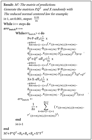
Algorithm 1. Custom mini bath gradient descent.

• $B_o$ : vector which the average marks awarded to items;

• $B_u$ : vector which represents the average explicit user notes;

• $\mu$ : total average of items;

• $B_{\mu }$ : matrix with the element have the same value $\mu$ ;

• $ϵ$ : the tolerance strictly greater than 0 and very small;

• u represents a user; i represents an item; n represents the number of users;

• m represents the number of items;

• bs represents the size of batch;

• ${{\nabla }_x\left(f\right)|}_{x=a}$ is mathematical expression which means of f in x applied in a.

3.3. The Combination Approach

The recommendation system uses a combination of the probabilistic model and the matrix factorization approach. Before predicting an o item on a user u, the probabilistic model predicts $y_o\left(u\right)$ score; and the matrix factorization predicts $x_o\left(u\right)$ score. The combination will predict $z_o\left(u\right)$ score which consists of averaging all predicted scores for the recommendation of item o to user u (Algorithm 2).

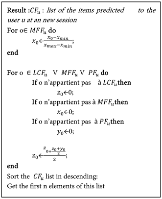
Algorithm 2. Top recommends.

While considering the following annotations:

• u: a user;

• o: an item;

• $MF{F}_u$ : list of the items predicted by the matrix factorization to the user u. We denote $x_o$ a score of item o of this list;

• $P{F}_u$ : list of the items predicted by the probabilistic model to the user u. We denote $y_o$ a score of item o of this list;

• $LC{F}_u$ : list of the items predicted by the combination approach to the user u at the last session. We denote $z_o$ a score of item o of this list;

• $C{F}_u$ : list of the items predicted by the combination approach to the user u at a new the session. We denote ${z^{\prime }}_o$ a score of item o of this list;

• $x_{\min }$ and $x_{\max }$ are the minimum and maximum value of $MF{F}_u$ respectively;

n is the number of top items to recommend to the user u.

4. Our Results

The quality of a recommendation algorithm can be evaluated using different types of measurement

• Statistical accuracy metrics, which evaluate the accuracy of a filtering technique by comparing the predicted ratings directly with the actual user rating. One most popular measures for estimating the accuracy of grade predictions is Root Squared Mean Error (RMSE). Let I be the set of items and U that of the users. Let $T\subset I$ be a test set of items, $p\left(u,i\right)$ a user note prediction u for item i and $n\left(u,i\right)$ the actual score assigned by the user u for the item i.

$\text{RMSE}=\sqrt{\frac{1}{card\left(T\right)}\times {\displaystyle {\sum }_{n\in U,i\in T}{\left(p\left(u,i\right)-n\left(u,i\right)\right)}^2}}$ [11] (12)

• Decisions support accuracy metrics. We focuse on the following metrics: accuracy, precision, recall and f1 Score. These metrics help users in selecting items that are of very high quality out of the available set of items. Table 1 represents the possible outcomes after the recommendation process is applied.

• Accuracy is a ratio of correctly predicted observations to the total observations. Precision is the ratio of correctly predicted positive observations to the total predicted positive observations. Recall is the ratio of correctly predicted positive observations to the total useful predicted observations and f1 Score is the weighted average of Precision and Recall.

$\text{accuracy}=\frac{\text{TP}+\text{TN}}{\text{TP}+\text{TN}+\text{FN}+\text{FP}}$ [11] (13)

$\text{precision}=\frac{\text{TP}}{\text{TP}+\text{FP}}$ [11] (14)

$\text{recall}=\frac{\text{TP}}{\text{TP}+\text{FN}}$ [11] (15)

$\text{f}1\text{Score}=\frac{2\times \text{recall}\times \text{precision}}{\text{recall}+\text{precision}}$ [11] (16)

The assessment of the resulting model is made solely by the model produced by the matrix factorization method. So the problem we encountered was in the number of latent vectors. The first problem concerns the RSME error as a function of the number of latent vectors. And the second concerns the RMSE error as a function of the number of learning iterations.

From Figure 1, it is clear that the lower the number of latent vectors, the better we have RMSE error (Root Mean Squared Error). In Figure 2, we visualize the error RMSE according to the number of iterations for 3 latent vectors after each 100 iterations. And in Figure 3, we visualize the error RMSE according to the number of iterations for 10 latent vectors after each 50 iterations. We observe these two figures, the diminution of the error. Also, this decrease is almost similar. But in Figure 1, we notice a better RMSE error for 3 latent vectors compared to 10 latent vectors. This leads us to fix the number of latent vectors at 3; which is a wise choice since the number of latent vectors chosen must be the smallest possible. Knowing that we have opted for 3 latent vectors, Figure 4 gives

Table 1. Outcomes after the applied of recommendation process.

Legend: Appreciated: properly predicted model; Not appreciated: improperly predicted model; Recommended: exact outcome; Not recommended: incorrect outcome.

Figure 1. RMSE according to the number of latent vectors.

Figure 2. RMSE based on the number of learning iterations for 3 latent vectors.

Figure 3. RMSE based on the number of learning iterations for 10 latent vectors.

Figure 4. Value between 0 and 1 depending on the type of evaluation measures for 3 latent vectors.

us the evaluation measures for this collaborative filtering. We find better values for rmse, precision, recall and f1 score. The evaluation measure accuracy is bad because the matrix factorization method merely predicts a matrix so as to minimize a certain error. So it is possible to find no good prediction since this method is concerned to minimize a certain error in a local minimum.

5. Discussion

In the family of collaborative filtering techniques in recommender systems, the most popular is the matrix factorization technique. Most of the time, a bias is added to the technique. This bias is to adjust the fact that some users give ratings more elevated than others and also the fact that some items have more ratings than others [16]. In this work, we suggested a combination of a matrix factorization algorithm with a bias like the one used in [16] to a probabilistic model. This aims to get the best of both of these techniques in order to improve the recommendation accuracy. We got a better result than the matrix factorization alone, but we need to improve our probabilistic model in order to consider more events from the user or to get a better estimation of the law followed by those events.

6. Conclusion

In this paper, we suggested a combination of two standard approaches to recommender systems in order to improve the accuracy of their predictions. Indeed, we got better results than the standard techniques that we combined which were the matrix factorization and a probabilistic model. However, this work has some limitations. In fact, the set of events used to compute the probability in our probabilistic model is not a full set of events and also a parallelization of our matrix factorization algorithm could reduce the execution time.

Acknowledgements

We also thank Pr. Thomas BOUETOU BOUETOU, head of the Department of Computer Engineering for providing us with an adequate working area. We also thank the anonymous referees for their useful suggestions.

Conflicts of Interest

The authors declare no conflicts of interest regarding the publication of this paper.

References

[1]	Betru, B.T., Onana, C.A. and Batchakui, B. (2017) Deep Learning Methods on Recommender System: A Survey of State-of-the-Art. International Journal of Computer Applications, 162, 17-22. https://doi.org/10.5120/ijca2017913361
[2]	Adomavicius, G. and Tuzhilin, A. (2005) Toward the Next Generation of Recommender Systems: A Survey of the State-of-the-Art and Possible Extensions. IEEE Trans, 17, 734-749. https://doi.org/10.1109/TKDE.2005.99
[3]	Salakhutdinov, R. and Mnih, A. (2007) Probabilistic Matrix Factorization. 20th International Conference on Neural Information Processing Systems, Vancouver, 3-6 December 2007.
[4]	Zoulla, D. (2019) Conception et Implémentation d’un Système de Recommendation de produits bancaires: Cas de Afriland First Bank. Master Thesis National Advanced School of Engineering of Yaoundé, Yaoundé, 55-57.
[5]	Li, Y.Y. and Li, Y. (2020) Study of Merchant Adoption in Mobile Payment System Based on Ensemble Learning. American Journal of Industrial and Business Management, 10, 861-875. https://doi.org/10.4236/ajibm.2020.105058
[6]	Nakamura, A. and Abe, N. (1998) Collaborative Filtering Using Weighted Majority Prediction Algorithms. 15th International Conference on Machine Learning, Madison, 24-27 July 1998, 395-403.
[7]	Breese, J.S., Heckerman, D. and Kadie, C. (1998) Empirical Analysis of Predictive Algorithms for Collaborative Filtering. Proceedings of the 14th conference on Uncertainty in Artificial Intelligence, Madison, 24-26 July 1998, 43-52.
[8]	Felfernig, A., Friedrich, G., Jannach, D. and Zanker, M. (2011) Recommender Systems, an Introduction. Cambridge University press, Cambridge, 335.
[9]	Zhu, L. and Yang, Y. (2015) Refine Item-Based Collaborative Filtering Algorithms with Skew Amplificatio. College of Computer Science and Technology, Shanghai University of Electric Power, Shanghai.
[10]	Basu, C., Hirsh, H. and Cohen, W. (1998) Recommendation as Classification: Using Social and Content-Based Information in Recommendation. Association for the Advancement of Artificial Intelligence, Menlo Park.
[11]	Isinkaye, F.O., Folajimi, Y.O. and Ojokoh, B.A. (2015) Recommendation Systems: Principles, Methods and Evaluation. Egyptian Informatics Journal, 16, 261-273. https://doi.org/10.1016/j.eij.2015.06.005
[12]	Zheng, L. (2015) A Survey and Critique of Deep Learning on Recommender Systems. University of Illinois at Chicago, Chicago.
[13]	Koren, Y., Bell, R. and Volinsk, C. (2009) Matrix Factorization Techniques for Recommender Systems. Computer, 42, 30-37. https://doi.org/10.1109/MC.2009.263
[14]	Lian, D., Zhao, C., Xie, X., Sun, G., Chen, E. and Rui, Y. (2014) GeoMF: Joint Geographical Modeling and Matrix Factorization for Point-of-Interest Recommendation. Proceedings of the 20th ACM SIGKDD International Conference on Knowledge Discovery and Data Mining, New York, 24-27 August 2014, 831-840. https://doi.org/10.1145/2623330.2623638
[15]	Ivis, F. (2006) Calculating Geographic Distance: Concepts and Methods. NESUG 2006, Philadelphia, 17-20 September 2006, Article No. DA15.
[16]	Su, D., Cui, Z., Wu, J. and Zhao, P. (2013) Pre-Filling Collaborative Filtering Algorithm Based on Matrix Factorization. Applied Mechanics and Materials, 411-414, 2223-2228. https://doi.org/10.4028/www.scientific.net/AMM.411-414.2223