Advanced Transformation Technique to Solve Multi-Objective Optimization Problems

Margia Yesmin¹, Md. Abdul Alim²

¹Department of Mathematics and Statistics, Bangladesh University of Textiles, Dhaka, Bangladesh.
²Department of Mathematics, Bangladesh University of Engineering and Technology, Dhaka, Bangladesh.

DOI: 10.4236/ajor.2021.113010                

Abstract

Multi-objective optimization problem (MOOP) is an important class of optimization problem that ensures users to model a large variety of real world applications. In this paper an advanced transformation technique has been proposed to solve MOOP. An algorithm is suggested and the computer application of algorithm has been demonstrated by a flow chart. This method is comparatively easy to calculate. Applying on different types of examples, the result indicates that the proposed method gives better solution than other methods and it is less time consuming. Physical presentation and data analysis represent the worth of the method more compactly.

Keywords

MOOP, Harmonic Average Technique, Modified Harmonic Average Technique, Advanced Transformation Technique

1. Introduction

Multi-objective optimization (MOO) is an effective technique for studying optimal trade off solutions that balance several criteria. The fundamentals and applications of MOO have been already explored in great detail [1]. The main limitation of MOO is that its computational burden grows in size with the number of objectives. Various types of solution procedure have been already developed for solving MOO problems [2] - [21]. Some of them deal with theory and some of them concern with solution methods and applications.

To solve multi-objective linear programming problems, various types of methods have been proposed by various scholars, such as Mean and median method by Sulaiman and Sadiq [17], Optimal transformation technique by Sulaiman and Ameen [4], Harmonic mean by Sulaiman and Mustafa [9], New statistical average method by Nahar and Alim [12].

On the other hand, Linear fractional programming problem has been solved by different researchers by different techniques, for example, A new procedure proposed by Tantawy [3] and by Guzel [5], An improved method by Mehdi, Chergui and Abbas [7], Arithmetic average technique by Sulaiman, Sadiq and Rahim [8], A new approach presented by Akter and Modi [10], New geometric average technique proposed by Nahar and Alim [11].

Many research scholars have solved multi-objective quadratic programming problem by applying several methods. We include some of them. Optimal cutting plane procedure [19] and Arithmetic average transformation technique [20] had been used by Sulaiman and Rahim. Optimal average maximum-minimum technique and Optimal geometric average technique had been used by Sulaiman-Nawkhass [6] and by Sulaiman-Abdull [21] gradually to solve multi-objective quadratic programming problem.

The larger the size of the problem, the greater the number of inefficient solution generated and thus the slower the convergence of the algorithm. To overcome this problem, we propose an advanced transformation technique. We test the capabilities of this proposed technique drawing a comparison with other techniques.

In this paper, we focus our interest on multi-objective quadratic programming problem (MOQPP) where several quadratic objectives are to be optimized subject to a set of linear constraints and nonnegative integer variables. The optimization software package, namely AMPL has been employed in the computation.

Sen proposed a method of multi-objective programming for achieving several conflicting objectives simultaneously [1] [15]. Multi-objective linear programming problem (MOLPP) has been solved by many research scholars. Sulaiman and Sadiq had solved MOLPP by using mean and median [17]. Hamad-Amin used arithmetic average technique to solve it [18]. New statistical (arithmetic, geometric, harmonic) average techniques had been proposed by Nahar and Alim for solving MOLPP. Sulaiman and Rahim used optimal cutting plane procedure to solve MOQPP [19]. Arithmetic average transformation technique and Geometric average technique had been used by Sulaiman, Rahim and Sulaiman, Abdullah to generate efficient solutions of MOQPP [20] [21]. Yesmin and Alim suggested a modified harmonic average technique to get more accurate solution by solving MOQPP [15].

This study has presented MOQPP and proposed an advanced transformation technique to solve it. The result is compared with two different techniques such as harmonic average technique and modified harmonic average technique. The comparison table shows the effectiveness of the proposed method. The proposed technique is easier to realize and less time consuming. No matter how complex the problem, this proposed method can be applied. Physical interpretations have been presented and data analysis has been discussed for more convenience.

2. Multi-Objective Optimization Problem

Multi-objective optimization is an area of multiple criteria decision making that is concerned with mathematical optimization problems involving more than one objective function to be optimized simultaneously.

Mathematically, multi-objective decision making problems can be expressed as:

$\text{Max}/\text{Min}\left[f_1\left(x\right),f_2\left(x\right),\cdots ,f_k\left(x\right)\right]$

Subject to

$x\in X=\left\{x|g_h\left(x\right):\left\{\ge ,=,\le \right\}0,h=1,2,\cdots ,m\right\}$

where, $f_j\left(x\right)=\text{Objective for maximization},j\in J$

$f_i\left(x\right)=\text{Objective for minimization},i\in I$

The problem consists of n decision variables, m constraints and k objectives. $f_j\left(x\right),f_i\left(x\right)$ and $g_h\left(x\right)\forall i,j,h$ might be linear or nonlinear.

Mathematically, the multi-objective linear programming problem (MOLPP) can be defined as:

$\text{Max}/\text{Min}{f}_i=C_{i}x+{\alpha }_i,$

And mathematically the multi-objective quadratic programming problem (MOQPP) can be stated as:

$\text{Max}/\text{Min}{f}_i=\frac{1}{2}{x}^{\text{T}}{P}_{i}x+C_i^{\text{T}}x$

Subject to

$Ax\left[\begin{array}{c}\le \\ \begin{array}{c}=\\ \ge \end{array}\end{array}\right]B$

$x\ge 0$

$i=1,\cdots ,r$ for maximization and $i=r+1,\cdots ,s$ for minimization

where x is an n-dimensional vector of decision variables, P is a $\left(n\times n\right)$ symmetric matrix of coefficients. A is $\left(m\times n\right)$ matrix of coefficients, B and C are n-dimensional vector of constants. ${\alpha }_i\left(i=1,\cdots ,s\right)$ are scalar constants. All vectors are assumed to be column vectors unless transposed.

3. Techniques for Solving MOOP

3.1. Chandra Sen’s Approach

A multi-objective programming (MOP) is formulated and optimized under common constraints. The mathematical form of MOP is described as:

$\text{Optimize}Z=\left[\text{Max}{z}_1,\text{Max}{z}_2,\cdots ,\text{Max}{z}_r,\text{Min}{z}_{r+1},\cdots ,\text{Min}{z}_s\right]$

Subject to

$Ax\left[\begin{array}{c}\le \\ \begin{array}{c}=\\ \ge \end{array}\end{array}\right]b$

$x\ge 0$ (3.1)

In this method, all objective functions need to be maximized or minimized individually by Simplex method or by any other method. By doing this the individual optima are obtained for each objective function separately as:

$z_{\text{optima}}=\left\{{\alpha }_1,{\alpha }_2,\cdots ,{\alpha }_s\right\}$

The optimum value of the objective function ${\alpha }_i\left(i=1,2,\cdots ,s\right)$ may be positive or negative.

These values are used to form a single objective function by adding (maximum values) and subtracting (minimum values) of each result then dividing each $z_i$ by ${\alpha }_i$. The function is formulated as:

$\text{Max}Z=\underset{i=1}{\overset{r}{{\displaystyle \sum }}}\frac{z_i}{{\alpha }_i}-\underset{i=r+1}{\overset{s}{{\displaystyle \sum }}}\frac{z_i}{{\alpha }_i}$

Subject to the same constraints as Equation (3.1).

To make the objective function dimension free, the integrated objective function was summarized by weighting each objective function by inverse of its optima. Hence the integrated objective function is formulated without facing any complex with objective functions of different dimensions.

Then the single objective optimization problem is solved by simplex method. This method is known as Chandra Sen’s approach.

3.2. Harmonic Average Technique

Harmonic Mean: Harmonic mean of a set of observations is defined as the reciprocal of the arithmetic average of the reciprocal of the given values. If $x_1,x_2,\cdots ,x_n$ are n observations then

Harmonic Mean (HM) = $\frac{n}{{\displaystyle {\sum }_{i=1}^n\left(\frac{1}{x_i}\right)}}$

It provides a more reliable result when the results to be achieved are the same for the various mean adopted.

The steps to calculate the harmonic mean are as follows:

Step 1: Finding the reciprocal of the given values.

Step 2: Calculating the average for the reciprocals obtained in step 1.

Step 3: Finally calculate the reciprocal of the average obtained from step 2.

Multi-objective optimization problem given in (3.1) can be translated by harmonic average technique as:

$\text{Max}Z=\frac{{\displaystyle {\sum }_{i=1}^r{z}_i}}{H{M}_1}-\frac{{\displaystyle {\sum }_{i=r+1}^s{z}_i}}{H{M}_2}$

where, $H{M}_1=\frac{r}{{\displaystyle {\sum }_{i=1}^r\left(1/{\alpha }_i\right)}}$, $H{M}_2=\frac{s-r}{{\displaystyle {\sum }_{i=r+1}^s\left(1/{\alpha }_i\right)}}$.

Subject to same constraints as Equation (3.1).

$H{M}_1$ is the value of harmonic mean of maximized ${\alpha }_i\left(i=1,2,\cdots ,r\right)$ and $H{M}_2$ is the value of harmonic mean of minimized ${\alpha }_i\left(i=r+1,\cdots ,s\right)$. The values of $H{M}_1$ and $H{M}_2$ may be positive or negative. If they are negative we consider the absolute values of $H{M}_1$ and $H{M}_2$.

Some difficulties occur when calculating with harmonic mean. The harmonic mean is greatly affected by the values of the extreme items. It can’t be able to calculate if any of the item is zero. This calculation is cumbersome as it involves the calculation using reciprocals of the items.

3.3. Modified Harmonic Average Technique

According to modified harmonic average technique multi-objective optimization problem given in (3.1) can be converted into a single objective function as:

$\text{Max}Z=\frac{{\displaystyle {\sum }_{i=1}^r{z}_i}-{\displaystyle {\sum }_{i=r+1}^s{z}_i}}{HM}$

where

$HM=\frac{2}{\frac{1}{H{m}_1}+\frac{1}{H{m}_2}}$

and

$H{m}_1=\min \left\{{\alpha }_i;\left(i=1,2,\cdots ,r\right)\right\}$,

$H{m}_2=\min \left\{{\alpha }_i;\left(i=r+1,\cdots ,s\right)\right\}$

Subject to same constraints as Equation (3.1).

$H{m}_1$ is the minimum value of maximized ${\alpha }_i\left(i=1,2,\cdots ,r\right)$ and $H{m}_2$ is the minimum value of minimized ${\alpha }_i\left(i=r+1,\cdots ,s\right)$. The steps to calculate the harmonic mean are as follows:

Step 1: Find the minimum optimal value of the maximization problems.

Step 2: Find the minimum optimal value of the minimization problems.

Step 3: Calculate the average for the reciprocals obtained in step 1 and step 2.

Step 4: Finally calculate the reciprocal of the average obtained from step 3.

Modified harmonic average technique gives better solution than harmonic average technique.

4. Advanced Transformation Technique

Multi-objective optimization problem can be defined as:

$\text{Max}/\text{Min}\left[z_1,z_2,\cdots ,z_s\right]$

Subject to

$Ax\left\{\ge ,=,\le \right\}b,x\ge 0$ (4.1)

Suppose we optimize all the objective functions individually and obtain the values

$\text{Max}{z}_1={\alpha }_1$

$\text{Max}{z}_2={\alpha }_2$

$⋮$

$\text{Max}{z}_r={\alpha }_r$

$\text{Min}{z}_{r+1}={\alpha }_{r+1}$

$⋮$

$\text{Min}{z}_s={\alpha }_s$

where ${\alpha }_i$ are the values of objective functions.

We require the common set of decision variables to be the best compromising optimal solution. Here we can determine the common set of decision variables from the following combined objective function.

By our proposed Advanced transformation technique, we can obtain the single objective function as follows:

$\text{Max}Z=\frac{{\displaystyle {\sum }_{i=1}^r{z}_i}-{\displaystyle {\sum }_{i=r+1}^s{z}_i}}{O_{AT}}$

where $O_{AT}=\frac{1}{1/m}$ and $m=\min \left\{m_1,m_2\right\}$.

where $m_1=\min \left\{{\alpha }_i\right\},\forall i=1,\cdots ,r$.

$m_2=\min \left\{{\alpha }_i\right\},\forall i=r+1,\cdots ,s$

Subject to the same constraints as mentioned in (4.1).

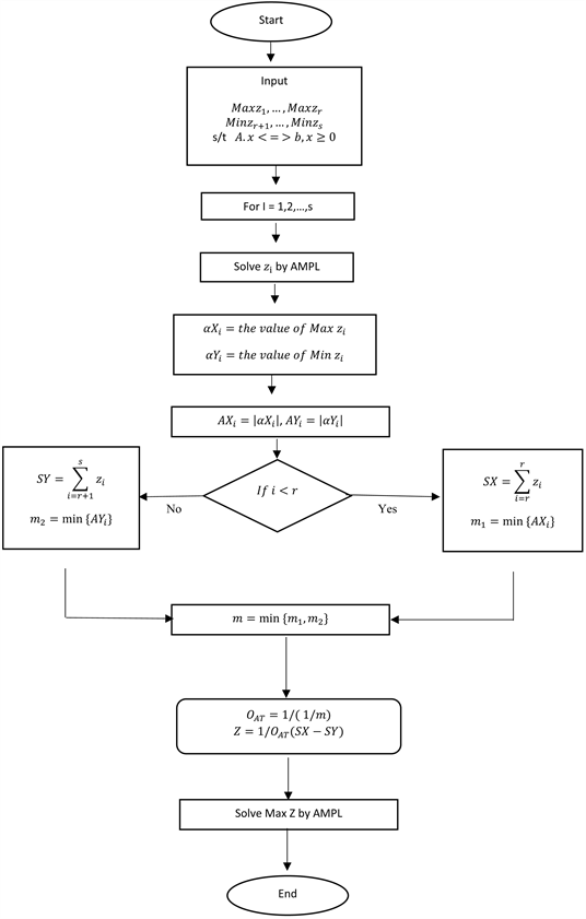
4.1. Algorithm

Step 1: Find the value of each objective function which is to be maximized or minimized.

Step 2: Solve the first objective function by mathematical programming language AMPL.

Step 3: Assign a name to the optimum value of first objective function $z_1$ by ${\alpha }_1$.

Step 4: Repeat step-2 for $i=2,3,\cdots ,s$.

Step 5: Select $m_1=\min \left\{{\alpha }_i\right\},\forall i=1,\cdots ,r$ and $m_2=\min \left\{{\alpha }_i\right\},\forall i=r+1,\cdots ,s$.

Step 6: Select $m=\min \left\{m_1,m_2\right\}$ and calculate $O_{AT}=\frac{1}{1/m}$.

Step 7: Optimize the combined objective function as $\text{Max}Z=\frac{{\displaystyle {\sum }_{i=1}^r{z}_i}-{\displaystyle {\sum }_{i=r+1}^s{z}_i}}{O_{AT}}.$

Under the same constraints by repeating Steps 2 & 3.

4.2. Flow Chart

5. Numerical Example

Consider the following Multi-Objective Quadratic Programming problem with linear constraints:

$\text{Max}{Z}_1=4x_1+2x_2-x_1^2-x_2^2+5$

$\text{Max}{Z}_2=2x_1+x_2-x_1^2$

$\text{Min}{Z}_3=6-6x_1+2x_1^2-2x_1{x}_2+2x_2^2$

$\text{Min}{Z}_4=2x_1+3x_2-2x_1^2$

$\text{s/t}{x}_1+4x_2\le 9$

$x_1+x_2\le 3$

$3x_1+2x_2\le 8$

$x_1,x_2\ge 0$

• AMPL:

After finding the value of each of individual objective functions by using AMPL, the numerical results are given in Table 1.

Table 1. Numerical results for given example.

• Chandra Sen’s Techniques:

By Chandra Sen’s Approach,

$\text{Max}Z=\underset{k=1}{\overset{r}{{\displaystyle \sum }}}\frac{Z_k}{\left|{\phi }_k\right|}-\underset{k=r+1}{\overset{s}{{\displaystyle \sum }}}\frac{Z_k}{\left|{\phi }_k\right|}$

$\begin{array}{c}\text{Max}Z=\frac{Z_1}{{\phi }_1}+\frac{Z_2}{{\phi }_2}-\frac{Z_3}{{\phi }_3}-\frac{Z_4}{{\phi }_4}\\ =\frac{4x_1+2x_2-x_1^2-x_2^2+5}{10}+\frac{2x_1+x_2-x_1^2}{3.0156}\\ -\frac{6-6x_1+2x_1^2-2x_1{x}_2+2x_2^2}{15}-\frac{2x_1+3x_2-2x_1^2}{6.9453}\\ =1.1734x_1+0.0968x_2-0.2751x_1^2-0.2333x_2^2+0.1333x_1{x}_2+0.1\end{array}$

Using Chandra Sen’s Approach, the system becomes,

$\text{Max}Z=1.1734x_1+0.0968x_2-0.2751x_1^2-0.2333x_2^2+0.1333x_1{x}_2+0.1$

Subject to

$x_1+4x_2\le 9$

$x_1+x_2\le 3$

$3x_1+2x_2\le 8$

$x_1,x_2\ge 0$

After solving we get,

$Z_{\max }=1.50957\text{with}{x}_1=2.18077\&x_2=0.728841$

• Harmonic Average Technique:

Using Harmonic Average Approach,

$H.M\left(10,3.0156\right)=\frac{2}{\frac{1}{10}+\frac{1}{3.0156}}=4.6338$

$H.M\left(15,6.9\right)=\frac{2}{\frac{1}{15}+\frac{1}{6.9}}=9.4521$

$\begin{array}{c}\text{Max}Z=\frac{1}{4.6338}\left(Z_1+Z_2\right)-\frac{1}{9.4521}\left(Z_3+Z_4\right)\\ =1.718x_1+0.33x_2-0.4316x_1^2-0.7448x_2^2+0.2116x_1{x}_2+0.4442\end{array}$

Using Harmonic Average Approach, the system becomes,

$\text{Max}Z=1.718x_1+0.33x_2-0.4316x_1^2-0.7448x_2^2+0.2116x_1{x}_2+0.4442$

Subject to

$x_1+4x_2\le 9$

$x_1+x_2\le 3$

$3x_1+2x_2\le 8$

$x_1,x_2\ge 0$

Solving this, we get,

$Z_{\max }=2.35006\text{with}{x}_1=2.11834\&x_2=0.522449$

• Modified Harmonic Average Technique:

Using Modified Harmonic Average Approach,

$H.AV=\frac{2}{\frac{1}{m_1}+\frac{1}{m_2}}=\frac{2}{\frac{1}{3.0156}+\frac{1}{6.9}}=4.1969$

$\begin{array}{c}\text{Max}Z=\frac{1}{H.AV}\left(Z_1+Z_2-Z_3-Z_4\right)\\ =2.3827x_1-0.4765x_1^2-1.4296x_2^2+0.4765x_1{x}_2-0.2383\end{array}$

Thus the QPP becomes,

$\text{Max}Z=2.3827x_1-0.4765x_1^2-1.4296x_2^2+0.4765x_1{x}_2-0.2383$

Subject to

$x_1+4x_2\le 9$

$x_1+x_2\le 3$

$3x_1+2x_2\le 8$

Solving this, we get,

$Z_{\max }=2.85616\text{with}{x}_1=2.16219\&x_2=0.25671$

• Advanced Transformation Technique:

Using proposed technique, select

$m_1=\min \left\{10,3.0156\right\}=3.0156\text{and}{m}_2=\min \left\{15,6.9453\right\}=6.9453$

then $m=\min \left\{m_1,m_2\right\}=\mathrm{3.0156.}$

Now, we get, $O_{AT}=\frac{1}{1/m}=\mathrm{3.0156.}$

Thus the QPP becomes,

$\begin{array}{c}\text{Max}Z=\frac{1}{O_{AT}}\left(Z_1+Z_2-Z_3-Z_4\right)\\ =\frac{1}{3.0156}\left(10x_1-2x_1^2-3x_2^2+2x_1{x}_2-1\right)\\ =3.3x_1-0.66x_1^2-0.99x_2^2+0.66x_1{x}_2-0.33\end{array}$

The system,

$\text{Max}Z=3.3x_1-0.66x_1^2-0.99x_2^2+0.66x_1{x}_2-0.33$

Subject to

$x_1+4x_2\le 9$

$x_1+x_2\le 3$

$3x_1+2x_2\le 8$

After solving, we get the result,

$Z_{\max }=4.3\text{with}{x}_1=2.29\&x_2=0.55$

Table 2 summarizes the solutions of the MOQPP using different approaches.

Table 2. Comparison table for given example.

It shows that the solution of the objective functions improved when we used the proposed technique. Advanced transformation technique gives better solutions than others.

Physical Interpretation

In this optimization problem, a process is going to search a better procedure to find maximum value of a given MOQPP.

Figure 1 shows that, how the optimized results have improved after applying different techniques. Physical interpretation of the given MOQPP after applying different techniques.

Figure 1. Physical interpretation of given example.

For more convenience, it can be shown in Figure 2.

Figure 2. Comparison with different techniques.

6. Data Analysis

Consider, some set of numerical examples of multi-objective optimization problems:

Example 6a.

$\max z_1=-3x_1^2-3x_2^2-6x_1{x}_2+30x_1+30x_2-48$

$\max z_2=-4x_1^2-4x_2^2-8x_1{x}_2+38x_1+38x_2-48$

$\min z_3=2x_1^2+2x_2^2+4x_1{x}_2-20x_1-20x_2+32$

$\min z_4=5x_1^2+5x_2^2+10x_1{x}_2-42x_1-42x_2+34$

s/t $x_1+2x_2\le 7$

$5x_1+2x_2\le 11$

$3x_1+2x_2\le 10$

$x_1,x_2\ge 0$

Example 6b.

$\max z_1=-3x_2^2+36x_1+34x_2$

$\max z_2=-2x_1^2+32x_1+32x_2$

$\min z_3=4x_1^2-36x_1-32x_2$

$\min z_4=2x_1^2-34x_1-30x_2$

$\min z_5=3x_2^2+6x_1{x}_2-32x_1-32x_2$

s/t $x_1+2x_2\le 7$

$5x_1+2x_2\le 11$

$3x_1+2x_2\le 10$

$x_1,x_2\ge 0$

Example 6c.

$\max z_1=0.5x_1+0.66x_2+0.833x_3$

$\max z_2=0.25x_1+0.33x_2+0.415x_3$

$\min z_3=0.2x_1-0.34x_2-0.3x_3$

$\min z_4=0.3x_1-0.32x_2-0.32x_3$

s/t $3x_1+4x_2+2x_3\le 60$

$2x_1+x_2+2x_3\le 40$

$x_1+3x_2+2x_3\le 80$

Example 6d.

$\max z_1=x_1$

$\max z_2=2+x_1+2x_2$

$\max z_3=3+x_2$

$\min z_4=-3x_2$

$\min z_5=-x_1-3x_2$

s/t $2x_1+3x_2\le 6$

$x_1\le 4$

$x_1+2x_2\le 2$

Solving examples (6a), (6b), (6c), (6d) by using Chandra Sen’s technique, Harmonic average technique, modified harmonic average technique and Advanced transformation technique we get Table 3.

Table 3. Comparison table for different data values.

According to above table we can conclude that, Advanced transformation technique gives better optimal solution than other techniques whether the functions are linear or quadratic.

7. Conclusion

This paper discusses the importance of the proposed advanced transformation techniques to solve multi-objective optimization problems. This is a quick safe technique which makes large and complex problems more tractable and accurate. The structural analysis of three different techniques for finding a basic feasible solution is compared throughout performed numerical test examples. The study shows that the proposed method has better performance than other methods. Different data analysis and visual presentation ensure its perfection.

Conflicts of Interest

The authors declare no conflicts of interest regarding the publication of this paper.

References

[1]	Sen, C. (1983) A New Approach for Multi Objective Rural Development Planning. The Indian Economic Journal, 30, 91-96.
[2]	Caramia, M. and Dell’Olmo, P. (2008) Multi-Objective Management in Freight Logistics. Springer-Verlag, London. https://doi.org/10.1007/978-1-84800-382-8 http://www.springer.com/978-1-84800-381-1
[3]	Tantawy, S.F. (2008) A New Procedure for Solving Linear Fractional Programming Problem. Mathematical and Computer Modelling, 48, 969-973. http://www.elsevier.com/locate/mcm https://doi.org/10.1016/j.mcm.2007.12.007
[4]	Sulaiman, N.A. and Hamadameen (2008) Optimal Transformation Technique to Solve Multi Objective Linear Programming Problem. Journal of Kirkuk University-Scientific Studies, 3, 96-106.
[5]	Guzel, N. (2013) A Proposal to the Solution of Multi Objective Linear Fractional Programming Problem. Abstract and Applied Analysis, 2013, Article ID: 435030. https://doi.org/10.1155/2013/435030
[6]	Sulaiman, N.A. and Nawkhass, M. (2013) Transforming and Solving Multi Objective Quadratic Fractional Programming Problem by Optimal Average of Maximin and Minimax Techniques. American Journal of Operation Research, 3, 92-98. https://doi.org/10.14419/ijamr.v2i2.838
[7]	Mehdi, M., Chergui, M. and Abbas, M. (2014) An Improved Method for Solving Multi Objective Integer Linear Fractional Programming Problem. Advances in Decision Science, 2014, Article ID: 306456. https://doi.org/10.1155/2014/306456
[8]	Sulaiman, N.A., Sadiq, G.W. and Rahim, A. (2014) New Arithmetic Average Technique to Solve Multi Objective Linear Fractional Programming Problem and Comparison with Other Techniques. New Arithmetic Average Technique, 18, 122-131.
[9]	Sulaiman, N.A. and Mustafa, R.B. (2016) Using Harmonic Mean to Solve Multi Objective Linear Programming Problem. American Journal of Operation Research, 6, 25-30. https://doi.org/10.4236/ajor.2016.61004
[10]	Akter, H. and Moodi, G. (2017) An Approach for Solving Multi Objective Linear Fractional Programming Problem and Comparison with Other Techniques. International Journal of Scientific and Innovative Mathematical Research, 5, 1-5. https://doi.org/10.20431/2347-3142.0511001
[11]	Nahar, S. and Alim, A. (2017) A New Geometric Average Technique to Solve Solve Multi Objective Linear Fractional Programming Problem and Comparison with New Arithmetic Average Techniques. IOSR Journal of Mathematics, 13, 39-52.
[12]	Nahar, S. and Alim, A. (2017) A New Statistical Average Method to Solve Multi Objective Linear Programming Problem. International Journal of Science and Research, 6, 623-629.
[13]	Sulaiman, N.A. and Mustafa, R.B. (2016) Transform Extreme Point Multi Objective Linear Programming Problem to Extreme Point Single Objective Linear Programming Problem Using Harmonic Mean. Applied Mathematics, 6, 95-99.
[14]	Sohag, Z.I. and Asadujjaman, M. (2018) A Proposed New Average Method for Solving Multi Objective Linear Programming Problem Using Various Kinds of Mean Technique. Mathematics Letter, 4, 25-33. https://doi.org/10.11648/j.ml.20180402.11
[15]	Sen, C. (2018) Sen’s Multi Objective Programming Method and Comparison with Other Techniques. American Journal of Operation Research, 8, 10-13.
[16]	Yesmin, M. and Alim, A. (2020) A New Quadratic Formulation to Ensure Maximum Profit of a Textile Industry and a Modified Harmonic Average Technique to Solve MOQPP. International Journal of Science and Research, 9, 937-943.
[17]	Sulaiman, N.A. and Sadiq, G.W. (2006) Solving the Linear Multi-Objective Programming Problems: Using Mean and Median Value. Al-Rafiden Journal of computer sciences and mathematics, University of Mosul, 3, 69-83. https://doi.org/10.33899/csmj.2006.164037
[18]	Hamad-Amin, A.O. (2008) An Adaptive Arithmetic Average Transformation Technique for Solving MOOPP. MSc. Thesis, University of Koya, Koya.
[19]	Sulaiman, N.A. and Abdul-Rahim, B.K. (2011) Optimal Cutting Plane Procedure for Multi-Objective Quadratic Programming Problem. Journal of Koya University, No. 20, 119-130.
[20]	Sulaiman, N.A. and Abulrahim, B.K. (2013) Arithmetic Average Transformation Technique to solve Multi-Objective Quadratic Programming Problem. Journal of Zankoy Sulaimani-Part A, 15, 57-69. https://doi.org/10.17656/jzs.10233
[21]	Sulaiman, N.A., Abdullah, R.M. and Abdull, S.O. (2016) Using Optimal Geometric Average Technique to solve Extreme Point Multi-Objective Quadratic Programming Problem. Journal of Zankoy Sulaimani-Part A, 18, 63-72. https://doi.org/10.17656/jzs.10535