An Automatic Optimization Technique for the Calibration of a Physically Based Hydrological Rainfall-Runoff Model ()
1. Introduction
The modeling of the hydrological behaviour of the basins is essential in the problems related to the management of water resources, town and country planning or in another facet of hydrological risks [ Gnouma, 2006]. Hydrological models intervene in the prevision of hydrological variables, tanks management, decision taking or even in the improvement of the understanding of the rainfall-runoff processes [ Samah, 2017; Obada, 2017]. These tools are a set of mathematical equations that describe and represent in relatively simple way the hydrological processes occurring in a basin. Each model includes several parameters to describe the state of the system in question. Some of these parameters are conceptual or unavailable by direct measuring and are estimated from historical data before setting up the model. This parameter estimation process is called calibration. This task is complex and presents many difficulties due to the uncertainty related to the model structure, the model inputs and the output flow. The model calibration impacts on its reliability, its accuracy and its performance to reproduce the mechanism of the studied system and its predictions of the hydrological variables. The HyMoLAP model is one of the most recent hydrological models which continues to prove its performance [ Afouda et al., 2004; Afouda & Alamou, 2010]. Through a lot of satisfying works with the help of the manual and semi-automatic calibration approaches [ Alamou, 2011; Alamou et al., 2015]. This model will therefore be used, as reference, in the present work. One of the fundamental steps of the rainfall-runoff modeling is the calibration of the parameters of the model. There are two ways of calibrating a model: the manual and the automatic one. The automatic calibration of hydrological models presents the advantage of speed over the manual calibration mainly in the presence of a high number of parameters to be identified [ Dakhlaoui, 2014]. Its efficiency is measured in terms of the necessary time required to reach an optimal solution. It is therefore important to choose an algorithm that will permit to quickly find the optimum set of parameters. We choose the Downhill Simplex method also known as the Nelder-Mead Algorithm which is a local search method allowing to optimize (maximize or minimize) a function in a given domain which contributes to better refine the solution and to facilitate convergence. [ Dakhlaoui, 2014]. This algorithm has been implemented on the problems of rainfall-runoff calibration. In the case of a modeling, the function to minimize is a performance criterion performance: Nash Stuctliffe Efficiency (NSE), Root Mean Square Error (RMSE), coefficient of determination R2, Mean Absolute Error (MAE) or any function that can be used as performance criterion. Due to the fact that calibration impacts on the models quality, it is necessary to define an efficient and performant calibration strategy. This is the reason why the present study is being conducted.
2. Methodology
2.1. Field of Study and Data
At the scale of West Africa, Ouémé is a small coastal river that covers at Bonou, the most advanced hydrological station before the delta, an area of 46,990 km2. Oueme is the largest river of Benin and it springs from the classified forest of Tanéka (Atacora) [ Le Lay, 2006]. This is the largest river in Benin covering more than the third part of the territory. The Oueme at Beterou basin (09˚12'N; 02˚16'E) [ Alamou, 2011] is the area of interest of the present study. Its natural outlet, which is located at a few kilometers in the downstream of the confluence of Oueme with the Yérou Maro, is the station of Beterou created in 1952. The surface covered by Oueme is 10,475 km2 (Figure 1).
Data used in this study are: daily precipitation, daily potential evapotranspiration and hydrometric data. Precipitation and potential evapotranspiration over the period 1960-2014 are obtained from the Meteorology National Head office in Benin, while river discharge data are obtained from the National Directorate of Water in Benin.
2.2. Presentation of the HyMoLAP Model
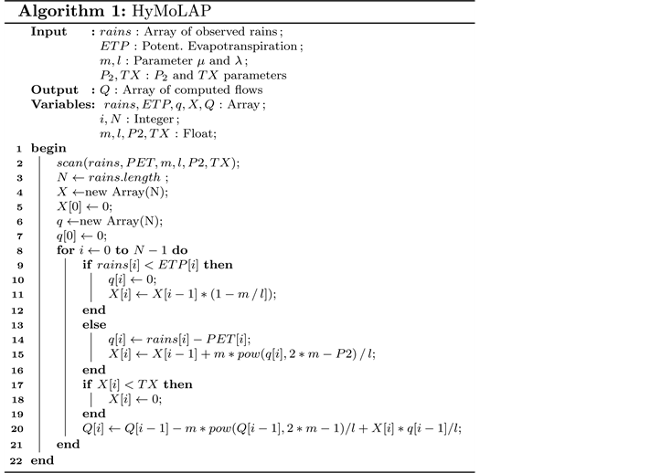
HyMoLAP is a physically based hydrologic model with two parameters. It is conceived from the Least Action Principle which uses the principle of minimum energy expenditure. This principle is expressed in the following words: Nature always follows the simplest ways.... and the simplest ways are those that minimize natural energy expenditure [ Afouda et al., 2004].
![]()
Figure 1. Geographic location of Oueme at Beterou basin.
The Least Action Principle was formulated at its origin by par (Maupertus, Euler, Lagrange, etc) and generalized in the twentieth century by Noether theorem. It has been largely applied in fundamental physics [ Arnold, 1974; Doubrovine et al., 1979] and is henceforth conceived as a universal mathematic law of the nature. The HyMoLAP Model comprises a production function (Equation (1)) and a transfer function (Equation (2)) provided by:
 (1)
(1)
 (2)
(2)
where Q is the river discharge at the outlet of the basin,  is a non linearity parameter,
  is the recession coefficient of the basin, q is to the difference between the rainfall and the potential evapotranspiration (PET) and is termed effective rainfall and t describes the model input.
Equation (1) describes explicitly the production process (i.e. the action of the unsaturated zone that accounts for evaporation and evapotranspiration and divides the resulting rainfall event into two components: overland and underground) and Equation (2) describes the transformation process (i.e. the process by which the rainfall volumes for the overland component and the underground component are transformed into runoff).
Figure 2 presents an algorithm on HyMoLAP Model. Xt is the state of soil at a date t, P2 and TX (minimum value of the ground state) are two constants.
2.3. Calibration
The goal of calibration is to set the value of parameters that we are unable to measure or estimate accurately. The choice of the value should be based on those which can permit the best agreement between simulations and observations [ Deraedt, 2011]. It is important to use the series of data which presents the greatest contrast in the values in order to cover the greatest number of river discharge [ Ambroise, 1999; Grayson & Blöschl, 2000]. This allows to limit extrapolation at maximum while using the model.
The capacity of a model, with a defined parameter set, to better simulate is determined by an objective function. Its role is to inform about the gap between simulation and observation. The most appropriate set of parameters is the one corresponding to the maximum (or minimum) of this function [ Ambroise, 1999]. In many cases, the calibration is done only on the river discharge at the outlet. The objective function can be multiple and include all the variables that we want to test [ Ambroise, 1999; Grayson & Blöschl, 2000].
Some functions enable a deep verification while others have a vision in the whole. The ideal calibration would be to start testing the model in a whole as it is easier to achieve and to end up with the deep verification which are more complex.
2.3.1. The Objective Functions Used
Performances analysis consists at comparing the measured river discharge to the calculated ones. Several objective functions are used; in this study, we have taken into account some performance criteria especially Nash Sutcliffe Efficiency (NSE), Root Mean Square Error (RMSE), Mean Absolute Error (MAE) and R square (R2). In this work, we will admit the following notations:
·  the observed river discharge on the day i
·  simulated river discharge on the day i
·  the average of the river discharge
· and n the total number of days.
Nash Sutcliffe Efficiency (NSE)
 (3)
(3)
The results will get better when the criterion NSE is coming near 1.
An efficiency inferior to zero (NSE < 0 for a comparison of daily river discharge indicates that the average observed is better predictor than the model. A value of NSE equal to 0.5 for a daily river discharge comparison is considered as an acceptable value in some hydrological studies [ Zhang et al., 2013; Waters et al., 2011; Moriasi et al., 2007].
Root Mean Square Error (RMSE)
It is given by Equation (4) and represents the quadratic difference mean between two series and the distance between the two series.
 (4)
(4)
When the RMSE is nearer to zero, the two considered series are similar.
Mean Absolute Error (MAE)
It is the mean absolute error and is given by Equation (5). It represents the absolute value of the average errors between the data of the two series taken two by two.
 (5)
(5)
Like the RMSE it is very closer to zero when the two considered series are similar.
Coefficient of determination (R2)
The measure R2 given by the formula 2.3.1 represents the square of the linear correlation coefficient between the observed river discharge and the simulated river discharge.

Many researchers like [ Moriasi et al., 2007] suggest all values of R2 superior to 0.5 for comparison of daily bit is a level acceptable in hydrologic simulation.
2.3.2. Research of the Set Optimal Parameter and Presentation of Nelder-Mead Algorithm
The research of the set optimal parameter may either be manual or automated. In this study, we will be interested in the automated research which consists of minimizing (the present case) or maximizing the objective function in a minimum number of iterations with the algorithm of auto-calibration. Here the algorithm of auto-calibration used is Nelder-Mead algorithm also known as Downhill Simplex Method.
The algorithm Downhill Simplex Method [ Nelder-Mead, 1965], is a non-linear optimization algorithm published by John Nelder and Roger Mead in 1965. It is a heuristic digital method which seeks to minimize a continuous function in a space of several dimensions. It exploits Simplexes concept which is a polytope of N + 1 summits I a space of N dimensions. Initially going from such a simplex, this goes through some simple changes in the course of the Iterations: it deforms, moves and reduces progressively till its summits come nearer to the point where the function is locally minimal. Calibration consists of using Nelder-Mead algorithm in order to get some sets of parameters in function with the different objective functions. Then these sets of parameters are sent to the model so as to obtain the calculated flows. These flows are added to the observed river discharge helping us to do simulations.
The algorithm is decomposed into many steps.
Step 1: Choose the summits of the initial simplexe S0.
Let’s consider a function f in a dimension space .
.
The algorithm begins by the choice of  points taken in this space with respective components
 . We obtain a set
 .
.
The image points of the elements of ![]() are the summits of
are the summits of![]() .
.
![]()
Step 2: Constructing the summits of the initial simplex S0 in a way that it is degenerated.
A consequence of the projection on the milestone is that the simplex can generate in the hyper plan some active milestones. If the simplex has converged with the active milestones, we can either have converged towards a local minimum or to a degenerated minimum (Figure 3), that is a minimum in the hyper plan.
This step consists in calculating the images by f of the elements of ![]() next to select them.
next to select them.
Then we construct the set ![]() so that
so that ![]() are selected.
are selected.
We pose![]() . We will call
. We will call![]() , the basis of the simplex
, the basis of the simplex![]() .
.
We pose: ![]() and
and![]() ,
, ![]() ,
, ![]() the points which components are respectively
the points which components are respectively![]() ,
, ![]() and
and![]() .
.
![]()
Step 3: Determination of the Centroid G of the polytope B ![]()
G is the centre of attraction of all the points of![]() . We then have:
. We then have:
![]()
![]()
Step 4: Reflection about G.
Let’s make ![]() the point of component
the point of component![]() .
.
This step consists of constructing![]() , so that
, so that
![]()
For the standard value![]() ,
, ![]() is the image of
is the image of ![]() by the cental symmetry of center G (Figure 4).
by the cental symmetry of center G (Figure 4).
We have:
![]()
![]()
Step 5: Determination of the new simplex S1
We distinguish four (4) possible cases:
Case n˚1: ![]()
The value of the function in ![]() is in the way that the one in
is in the way that the one in ![]() is more explicative than the one in
is more explicative than the one in![]() . We then proceed to the replacement of
. We then proceed to the replacement of ![]() by
by![]() . So we obtain a new simplex
. So we obtain a new simplex ![]() (Figure 5) then we return back to the Step 2.
(Figure 5) then we return back to the Step 2.
Case n˚2: ![]()
The value of the function in ![]() is less than the one in
is less than the one in ![]() so the simplex is stretched in that direction. We then do an expansion of the simplex by determining
so the simplex is stretched in that direction. We then do an expansion of the simplex by determining ![]() image of G by the central symmetric of
image of G by the central symmetric of ![]() (Figure 6). Then we get:
(Figure 6). Then we get:
![]()
The standard value of ![]() is 2 and the equation becomes
is 2 and the equation becomes
![]()
If![]() , we replace
, we replace ![]() by
by![]() . Else, we replace
. Else, we replace ![]() by
by ![]() and then we return back to the step 2.
and then we return back to the step 2.
Case n˚: ![]()
The value of the function in ![]() is better than the one of
is better than the one of![]() . Therefore,
. Therefore,
![]()
Figure 5. Construction of the new simplex.
the local look (aspect) of the function is a valley. We then proceed to a contraction of the simplex on itself in only one direction by determining the point Q (Figure 7) so that:
![]()
According to the value of![]() , the contraction may be either internal or external.For the particular value of
, the contraction may be either internal or external.For the particular value of![]() , Q is the middle of the segment
, Q is the middle of the segment![]() . We then have:
. We then have:
![]()
If![]() , we replace
, we replace ![]() by Q end go back to the step 2. If not we move to the case 4.
by Q end go back to the step 2. If not we move to the case 4.
Case n˚4: Contraction in all the directions
Figure 8: We construct the images of all the summits by the homothety of ratio ![]() by the centre
by the centre![]() . We then replace the components of each
. We then replace the components of each ![]() by:
by:
![]()
For![]() , all the points
, all the points ![]() is replaced by the middle of the segment
is replaced by the middle of the segment ![]() and we go back to the step 2.
and we go back to the step 2.
![]()
![]()
Figure 8. Contraction in all the directions.
![]()
The continuation of the algorithm consists in repeating the previous steps [ O’Neill, 1971] until we reach the fixed level as preliminary or reach the convergence towards an entire minimum [ Kelley, 1999a; Kelley, 1999b].
![]()
2.3.3. Calibration Technique
The calibration of the model with the objective function follows the following steps:
1) Calculate the final simplex from Nelder Mead algorithm, an initial simplex (from potential arbitrary values of the parameters) and an objective function.
final_simplex:= nelder_mead(init_simplex, obj_funct)
2) Calculate the simulated river discharge by applying HyMoLAP algorithm on the final simplex (parameters values).
q_sim:= HyMoLAP(final_simplex)
3) Set out the curve simulating the observed river discharge and the simulated ones.
The implementation of the objective functions for the use of Nelder Mead algorithm may sometimes show itself delicate. In fact, Nelder Mead algorithm tries to minimize the values of the used objective function. Yet,
![]()
In this case, the algorithm of Nelder Mead must maximize the values of NSE. This comes to minimize the function![]() .
.
![]()
2.4. Validation
Validation is the step that enables to make sure of the model quality. In fact, calibration permits to obtain a good set of parameters favoring then a good simulation of data. To guarantee that the simulation is still correct, we have to use another series of data. Besides a good set of parameters that has enabled to calibrate and validate a model is only used for a scope of application (basin, for the models rain debit or spatialized) well determined [ Grayson & Blöschl, 2000].
To carry out validation, it is necessary to have at disposal a series of data which has not been used while calibrating which corresponding output data are known. It will be used for simulating in the same side basin the parameters values got from calibration. The result is then compared to the reality with the same objective function as previously. For the spatialized models, the same approach may be achieved on another side basin [ Ambroise, 1999].
If the simulation results are not convincing, the parameter values and/or the structure of the model should be questioned [ Deraedt, 2011]. Poor and similar residues for calibration and validation are a sign that the model is correct [ Grayson & Blöschl, 2000]. It is possible to compare the efficiency of many models from the value of the objective functions but only for the same side basin and the same period of time [ Ambroise, 1999].
It is strongly advised to work out of the conditions of validation When using the calibrated and validated model [ Ambroise, 1999].
2.5. Development Environment
All the implementations achieved in the frame of this work are carried out under the Python language.
In fact, several packages exist under Python to optimize the set of data to be used in parameters for some objective functions. We have retained in this article the bookshop SctPy that contains a lot of toolboxes devoted to the method of scientific calculations. Its different sub modules correspond to different scientific applications like interpolation, integration, optimization, image processing, statistic, special mathematic function methods.
The other Python libraries used in this paper are Pandas, Numpy and Matplotlib.
3. Results and Discussions
3.1. Model Calibration and Validation
3.1.1. Calibration
The calibration was done during the period from 31/12/1964 to 30/12/1974.
Performance Criteria Values (PCV), parameters and constants obtained after the calibration of the model HyMoLAP are recorded in Table 1.
3.1.2. Validation
Validation was achieved in the period from 31/12/1974 to 30/12/1982.
Performance Criteria Values (PCV), parameters and constants obtained after the calibration of the model HyMoLAP are recorded in Table 2.
3.2. Technical Evaluation of the Model
The statistical results of the HyMoLAP model calibration and validation performance criteria (Table 1 and Table 2) and the graphical results of the calibration (Figure 9 and Figure 10) and validation (Figure 11 and Figure 12) indicated adequate calibration and validation over the flow range, although the calibration results showed better agreement than the validation results. The analysis in Table 1 shows that the model has very good calibration results. Indeed, the
![]()
Table 1. Values obtained after calibration.
![]()
Table 2. Values obtained after validation.
![]()
Figure 9. Simulation—Objective function: NSE.
![]()
Figure 10. Simulation—Objective function: MAE.
![]()
Figure 11. Validation—Objective function: NSE.
![]()
Figure 12. Validation—Objective function: MAE.
Nash criteria (NSE) and coefficients of determination R2 are 0.90 and 0.75 respectively in calibration and validation for the data used. The model having presented very good performance in calibration with NSEs and R2 greater than 0.5, which is an acceptable threshold in rainfall-runoff modeling at the daily scale according to [ Moriasi et al., 2007].
The simulated values were in good and very good ranges during validation for the sub-basin. In addition, the RMSE and MAE values, close to 0, obtained (RMSE between 0.33 and 0.53 and MAE between 0.34 and 0.54), confirm a similarity between observed and simulated river discharge for the model (Table 1 and Table 2). Since the objective Nash function has a value greater than 0.60, the simulation cannot be considered unsatisfactory. [ Ardoin-Bardin, 2004], but the degree of freedom of this function is not known. It was therefore supplemented by the correlation coefficient to confirm the quality of the data used (Figures 13-15) shows a strong relationship between these data.
3.3. Evaluation of the Impact of the Model Structure and Parameter Values on the Quality of the Simulations
The values of the objective functions obtained from the calibration are within the acceptable data ranges. It can be deduced from this that the set of parameters obtained will allow efficient simulations to be carried out.
The results obtained after validation using directly the parameter values obtained during validation are not very satisfactory as shown by the objective function values obtained.
Some factors have to be taken into account:
· the structure of the model;
· the parameter’s values.
The HyMoLAP model is a model based on a relationship between the observed river discharge at different dates (t) and the river discharge of the previous days
![]()
Figure 13. Linear correlation between observed river discharge.
![]()
Figure 14. Linear correlation between the calculated river discharge.
![]()
Figure 15. Linear correlation between observed and calculated river discharge.
(t − 1). The structure of the model would have to be questioned if the correlation between the river discharge rates calculated at the different dates t and calculated river discharge on dates t − 1 is not retained.
From Figure 13 and Figure 14 it can be concluded that the correlation is maintained by switching from observed to simulated river discharge. This allows us to deduce that the structure of the model is valid.
The values of the parameters depend intimately on the objective functions and the Nelder-Mead algorithm.
The Nelder-Mead algorithm is a heuristic numerical method that seeks to minimize the objective function and therefore does not go through all the possible values. It may happen that the optimal set of parameters is not reached. Nevertheless the results obtained are acceptable for calibration. For the validation on the other hand, the results seem slightly below what we expected. But Figure 15 shows us that the correlation coefficient between the observed and simulated river discharge rates is (r = 0.89), which is high and significant. This indicates that the peaks could be caused by the slow rise in water levels linked to soil saturation rather than by isolated precipitation episodes, which is similar to what has been observed in the oueme basin by [ Ardoin-Bardin, 2004]. The imperfections noted during the validation are thus probably more related to climatic variations and external factors (outliers) but we do not exclude the possibility that a better minimization algorithm would have given better results. We thus put into perspective the study of new optimization algorithms for hydrological modeling with HyMoLAP.
4. Conclusion and Perspectives
In this paper, we presented an approach that consists of automatically determining the optimal set for the calibration of the HyMoLAP model (which is a Based Global Hydrological Rainfall-Runoff Model) using the Downhill Simplex algorithm, tested on data from the Beterou basin. Through this research, we have brought some elements to problems related to the automatic choice of the optimal dataset using a non-linear optimization algorithm. We have shown that it is possible to find the set of parameters by exploiting the concept of simplex which is a polytope of N + 1 vertices in space with N dimensions. The quality of the sets of parameters obtained seems good enough to enrich the performance of the objective functions in a minimum number of iterations. We have analyzed the algorithm from a technical point of view, and we have performed an experimental comparison between some factors such as the structure of the model and the values of the parameters. The results of the algorithm are promising but they need to be refined or completed often. This analysis also allowed us to show how the algorithm minimizes objective functions.
In the future, we plan to apply the Nelder-Mead algorithm to other basins using more performance criteria in order to validate its efficiency in hydrological modeling. This will allow us to infirm or confirm the need to experiment with other approaches to determine the set of optimal parameters such as the use of combinatorial optimization or machine learning algorithms.