Outlier Detection and Effects on Modeling

Christopher O. Arimie¹, Emmanuel O. Biu², Maxwell A. Ijomah²

¹Department of Radiology, University of Port Harcourt Teaching Hospital, Port Harcourt, Nigeria.
²Department of Mathematics and Statistics, University of Port Harcourt, Port Harcourt, Nigeria.

DOI: 10.4236/oalib.1106619                

Abstract

In this work, a comprehensive framework for traditional outlier detection techniques based on simple and multiple linear regression models was studied. Two data sets were used for the illustration and evaluation of each class of outlier detection techniques (analytical and graphical methods). Outlier detection aims at identifying such outlier in order to improve the analytic of data and suitable model built. Furthermore, comparisons of the different methods were done to highlight the advantages, disadvantages and performance issues of each class of outlier detection techniques. The results show that by removing the influential points (or outliers), the model adequacy increased (from R2 = 0.72 to R2 = 0.97). It was observed that Jackknife residuals and Atkinson’s measure methods are very useful in detecting outliers; hence, both methods were recommended for outliers’ detection.

Keywords

Outliers’ Detection, Classification and Comparisons, Simple and Multiple Linear Regression Models

1. Background of the Study

Outliers are observations that appear inconsistent with the remainder of the dataset. Bollen and Jackman [1] defined outliers as observations that are distinct from most of the data points in the sample. Hawkins [2] described outlier as an observation that deviates so much from other observations as to arouse suspicions that it was generated by different mechanisms. Dixon [3] sees outlier as values that are dubious in the eyes of the researcher and contaminants. Outliers are often present in real data but may go unnoticed because nowadays much data are produced by computer without careful inspection or screening. Outliers may be mistakes in data entry or otherwise, accurate but unexpected observations which could shed new light on the phenomenon under study.

In general, outliers can be classified into two types: man-made one and random one. Man-made outliers may arise because of typographical error(s), misreporting of information, incorrect distribution assumption and sampling error. Random outliers, on the other hand, may arise because of random chance for drawing sample from a population. Presence of man-made or random outliers or both would seriously influence the result of statistical analysis including point and interval estimates and type 1 and type 11 errors. Outlier can cause us to misinterpret patterns in plots; it can affect visual resolution of remaining data in plot (forces observations into clusters) and may indicate that our model fails to capture important characteristics of the data. Unusual cases can substantially influence the fit of the ordinary least square model thus, leading to faulty conclusion. Some man-made outliers can be avoided by a strict data entry and rechecking process before conducting a statistical analysis. Data transformation is another way to reduce the influence of outliers (see Barnett and Lewis [4]; Montgomery [5]).

Quite a number of authors have proposed different methods of detecting outliers.

Abuzaid et al. [6], proposed a number of diagrammatical plots and hypothesis testing to detect outliers in the simple circular regression model. The work focused on detecting outlier in the down and Mardia’s circular-circular regression model. Zhang et al. [7] presented a method which applies signal processing techniques to solve important problems in data mining. They introduced an outlier detection approach termed to find out, based on wavelet transform. The main idea in the method is to remove the clusters from the original data and then identify the outliers. Rousseeuw [8] proposed a depth based method to detect outlier. The data points are organized in layers in the data space according to the value of the point depth. Aggarwal and Yu [9] proposed a method which entails studying the projection from the rest of the data in a sparse data with high dimensionality. Arning et al. [10] introduced a method which relies on the observations such that after seeing a series of similar data, an element disturbing the series is considered an outlier.

Hodge and Austin [11] identified an efficient method for on-line classification and outlier detection in multivariate sensor data. This involved a comparative review to identify and distinguish their advantages and disadvantages and introducing a survey of contemporary outlier detection techniques. Sebert et al. [12] and Montgomery [5] asserts that to identify the existence of outliers the standardized residuals are computed and a large standardized residual of (d > 3) indicates outlier. Worden et al. [13] used the concept of discordances to signal deviance from the norm.

Kitagawa [14] and Wing-Kam Fung and Bacon-Shone [15] applied Akaike information criterion (AIC) in detection of outliers by using (quasi) Bayesian approach with predictive likelihood. Belsey et al. [16] suggested standardizing each residual with an estimate of its standard deviation that is independent of the residual. This is accomplished by using as the estimate of variance for the i^th residual, the residual mean square from an analysis where that observation has been omitted. The result is a jackknife residual also called a fully studentized residual.

In this study, concentration is on the effect of outlier as well as detection methods on linear regression model. Specifically, we are concerned with observations that differ from the regression plane defined by the data. It is important to identify these types of outliers in regression modeling because the observations when undetected can lead to erroneous parameter estimates and inference from the model. Deleting outliers from a regression model can sometimes give completely different results as bias or distortion of estimates are removed. Identifying outliers in the real world data-base is important for improving the quality of original data and for reducing the impact of outliers. Identifying outliers and high-leverage points, is a fundamental step in the least-squares regression model building process. On this note, it is the purpose of this research to examine the effect of outliers on simple and multiple linear regression, compare different methods of detecting outlier and show its effect on modeling.

2. Methods of Outlier Detection and Effects on Regression Model

There are many methods for the detection of outliers in linear regression. They may be classified into graphical and analytical methods. The graphical methods include Scatter graph, Boxplot, Williams graph, Rankit graph (or Q-Q Plot) and graph of predicted residuals. The analytical methods are predicted residuals, standardized residuals, studentized residuals, Jack-knife residuals, Cook’s distance, Different-in-fits (DFFITS) and Atkinson’s measure.

The general linear model is given as

$y_{n\times 1}=X_{n\times k}{\beta }_{k\times 1}+{\epsilon }_{n\times 1}$ (2.1)

where,

$y_{n\times 1}$ is the observation (dependent variables);

$X_{n\times k}$ is the design matrix including a constant;

$\epsilon ~N\left(0,{\sigma }^{2}I\right)$ is the error term;

$\beta ={\left({\beta }_0,{\beta }_1,{\beta }_2,\cdots ,{\beta }_{k-1}\right)}^{\prime }$ is the coefficient and k is the number of covariates or predictors for each observation.

Then, the least square estimator is given as

$\beta ={\left(X^{\prime }X\right)}^{-1}\left(X^{\prime }Y\right)$ (2.2)

where the fitted (predicted) values for mean of Y are

$\hat{Y}={\rm X}\beta ={\rm X}{\left({{\rm X}}^{\prime }{\rm X}\right)}^{-1}\left({{\rm X}}^{\prime }Y\right)={\rm H}Y$ (2.3)

where $H=X{\left(X^{\prime }X\right)}^{-1}{X}^{\prime }$ is the projection matrix (or hat matrix).

The i^th diagonal element of H (given by $h_i={x^{\prime }}_i{\left({{\rm X}}^{\prime }{\rm X}\right)}^{-1}{x}_i$ is known as the leverage of the i^th observation).

Similarly, the i^th element of the residual vector

${\epsilon }_i=Y_i-{\hat{Y}}_i=\left(I-H\right)Y_i$ (2.4)

where H is as defined in Equation (2.3), I is the identity matrix and Y_i is corresponding fitted value ( $i=1,2,\cdots ,n$ ).

In this study, Outliers were detected using the following methods:

2.1. Studentized and Standardized Residuals

The Studentized residual is obtained by

${\epsilon }_{S.i}=\frac{{\stackrel{⌢}{\epsilon }}_i}{\hat{\sigma }\sqrt{1-h_i}}=\frac{{\stackrel{⌢}{\epsilon }}_i}{\sqrt{{\hat{\sigma }}^2\left(1-h_i\right)}}$ (2.5)

where $\hat{\sigma }$ is an appropriate estimate of $\sigma$, and the estimate of ${\hat{\sigma }}^2$ (Mean Residual Sum of Squares) is the internally studentized residuals. $h_i$ is leverage points as already defined.

${\hat{\sigma }}^2=\frac{1}{n-k}{\displaystyle \underset{j=1}{\overset{n}{\sum }}{\hat{\epsilon }}_j}$ (2.6)

where k is the number of parameters in the model (Equation (2.1)).

Studentized residuals with large absolute values are considered large. If the regression model is appropriate, with no outlying observations, each Studentized residual follows a t distribution with n − k − 1 degrees of freedom.

CRITICAL: Each deleted residual has a student’s t-distribution with n − k − 1 degrees of freedom.

If the Studentized residual is divided by the estimates of its standard error so that the outcome is a residual with zero mean and standard deviation one, it becomes standardized residual denoted by

${\epsilon }_{ST.i}=\frac{{\stackrel{⌢}{\epsilon }}_i}{sd\left(\sigma \right)}$ (2.7)

where $sd\left(\sigma \right)$ is the standard deviation of ${\hat{\sigma }}^2$ in Equation (2.6).

CRITICAL: The standardized residuals, d_i > 3 potentially indicate outlier.

2.2. Jackknife Residuals

The jackknife residuals are residuals which with an assumption of normality of errors have a student distribution with (n − k − 1) degrees of freedom. The formula is:

${\epsilon }_{J.i}={\stackrel{⌢}{\epsilon }}_{S.i}\sqrt{\frac{\left(n-k-1\right)}{\left(n-k-{\stackrel{⌢}{\epsilon }}^2{}_{S.i}\right)}}$ (2.8)

where ${\epsilon }_{S.i}$ is the Studentized residuals Equation (2.5).

The jackknife residual examines the influence of individual point on the mean quadratic error of prediction.

CRITICAL: Each deleted residual has a student’s t-distribution with n − k − 1 degrees of freedom.

2.3. Predicted Residuals

The predicted residual or Cross-validated residuals for observation i is defined as the residual for the i^th observation that results from dropping the i^th observation from the parameter estimates. The sum of squares of predicted residual errors is called the PRESS statistic:

${\epsilon }_{P.i}=\frac{{\epsilon }_i}{1-h_i}$ (2.9)

PRESS is called Prediction sum of squares; an assessment of your model’s predictive ability. PRESS, similar to the residual sum of squares, is the sum of squares of the prediction error. In least squares regression, PRESS is calculated with the following formula:

$\text{PRESS}={{\displaystyle \underset{i=1}{\overset{n}{\sum }}\left(\frac{{\epsilon }_i}{1-h_i}\right)}}^2$ (2.10)

where ${\epsilon }_i$ = residual and h_i = leverage value for the i^th observation. In general, the smaller the PRESS value, the better the model’s predictive ability.

2.4. Cook’s Distance

Cook’s distance D_i of observation, i is defined as the sum of all the changes in the regression model when observation i is removed from it. Cook [17] proposed a statistic for detection of outlier, given as:

$D_i=\frac{{{\displaystyle \underset{j=1}{\overset{n}{\sum }}\left(y_j-{\hat{y}}_{j\left(i\right)}\right)}}^2}{k{S}^2}$ (2.11)

and $S^2={\left(n-k\right)}^{-1}{\epsilon }^{\prime }\epsilon$ is the mean squared error of the regression model. Equivalently, it can be expressed using the leverage

$D_i=\frac{{\epsilon }_i^2}{k{S}^2}\left[\frac{h_i}{{\left(1-h_i\right)}^2}\right]$ (2.12)

Here, D_i measures the sum of squared changes in the predictions when observation “i” is not used in estimating $\beta$. D_i approximately follows F(p, n − p) distribution.

CRITICAL: The cut off value of Cook-Statistic is 4/n.

2.5. Difference-in-Fit (DFFIT)

It is the difference between the predicted responses from the model constructed using complete data and the predicted responses from the model constructed by setting the i^th observation aside. It is similar to cook’s distance. Unlike cook’s distance, it does not look at all of the predicted values with the i^th observation set aside. It looks only at the predicted values for the i^th observation. It combines leverage and studentized residual (deleted t residuals) values into one overall measure of how unusual an observation is. DFFIT is computed as follows:

$\text{DFFIT}={\epsilon }_i\left[\sqrt{\frac{n-k-1}{{\sigma }^2\left(1-h_i\right)-{\epsilon }_i^2}}\right]\sqrt{\frac{h_i}{1-h_i}}$ (2.13)

where ${\epsilon }_i$ = residual, n = sample size, k = the number of parameters in the model, σ² = variance and h_i = leverage value for the i^th observation.

CRITICAL: The cut off value of DFFIT is $2\sqrt{\frac{k}{n}}$.

2.6. Atkinson’s Measure (A_i)

It enhances the sensitivity of distance measures to high-leverage point. This modified version of cook’s measure D_i suggested by Atkinson is even more closely related to Belsey et al. (1980) [16] DFFITS and has the form

$A_i=\left|{\epsilon }_{J.i}\right|\left[\sqrt{\frac{n-k}{k}\times \frac{h_i}{1-h_i}}\right]$ (2.14)

where n, k, h_i are as defined in Equations (2.13) and ${\epsilon }_{J.i}$ is the absolute value of Jackknife residuals.

This measure is also convenient for graphical interpretation.

2.7. Scatter Graph and Box Plot

Scatter plot is a line of best fit (alternatively called “trendline”) drawn in order to study the relationship between the variables measured. For a set of data variables (dimensions) $X_1,X_2,\cdots ,X_k$, the scatter plot matrix shows all the pairwise scatter plots of the variables on the dependent variable.

A box plot is a method for graphically depicting groups of numerical data through their quartiles (i.e. Mean, Median Mode, quartiles). Box plots may also have lines extending vertically from the boxes (whiskers) indicating variability outside the upper and lower quartiles. It is also called box-and-whisker plot and box-and-whisker diagram. Outliers may be plotted as individual points and it can be used for outlier detection in regression model, where the primary aim here is not to fit a regression model but find out outliers using regression and to improve a regression model by removing the outliers.

2.8. Willams Graph, Rankit Graph (or Q-Q Plot) and Predicted Residuals Graph

The Williams graph (Williams [18]) has the diagonal elements H_ii on the x-axis and the jackknife residuals ${\hat{\epsilon }}_{Ji}$ on the y-axis. Two boundary lines are drawn, the first for outlier y = t_0.95(n − k − i), and the second for high leverages, x = 2k/n. Note: t_0.95(n − k − 1) is the 95% quantile of the student distribution with (n − k − 1) degrees of freedom.

The Q-Q plot (or Rankit Graph) has the quantile of the standardized normal distribution μp_i for $P_i=i/\left(n+\text{1}\right)$ on the x-axis and the ordered residuals ${\hat{\epsilon }}_{S.i},{\hat{\epsilon }}_{P.i},{\hat{\epsilon }}_{J.i}$ i.e. increasingly ordered values of various types of residuals on the y-axis.

The graph of predicted residuals (or Predicted Residuals Graph) has the predicted residuals ${\hat{\epsilon }}_{Pi}$ on the x-axis and the ordinary residuals ${\hat{\epsilon }}_i$ (Equation (3.4)) on the y-axis. The outlier can easily be detected by their location, as they lie outside the line y = x far from its central pattern (Meloun and Militky [19]).

3. Methodology

Two sets of data (see Appendix), were collected and used to build the regression models. The first was data of rainfall (in Millimetres) and yield of Wheat (in kg) and the second was data of agricultural products (Crop production, Livestock, Forestry and fishing) and Nigeria gross domestic product (GDP). The seven analytical and five graphical methods listed above were then applied to detect outliers in the simple and multiple linear regression models.

4. Results and Discussion

4.1. Simple Linear Regression

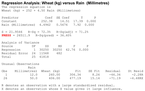
Simple linear regression of rainfall (Millimetres) on yield of Wheat (kg) was done, using Minitab 17 software to obtain the residuals of the model for outlier detection Methods to be applied.

4.1.1. Outlier Detection Methods

The seven analytical and five graphical methods for outlier detection discussed in Section 2 were used to detect outliers when the regression model was built using the rainfall and yield of wheat data. The results of the computation using the analytical methods are shown in Table 1 while Table 2 gives a summary of the number of outliers detected by each analytical method. Figures 1(a)-(f) show the scatter plot of outliers detected by the methods indicated. Figures 2(a)-(f) show the box plot of outliers detected by the methods indicated while Figures 3(a)-(d) show the Rankit Graph (or Q-Q Plot) of outliers detected.

(a)(b)(c)(d)(e)(f)

Figure 1. Scatter plots showing outliers detected by each of the analytical methods indicated. (a) Leveages; (b) Studentised residuals; (c) Cook’s distance; (d) Different-in-fits (DFFITS); (e) Jack-knife residuals; (f) Atkinson’s measure.

(a) (b) (c) (d) (e) (f)

Figure 2. Boxplots showing outliers detected by each of the analytical methods indicated. (a) Leverages; (b) Residuals; (c) Standardized residuals; (d) Atkinson’s measure; (e) Jack-knife residual; (f) Cook’s distance.

(a) (b) (c) (d)

Figure 3. Rankit graph (or Q-Q Plot) of outliers detected by each of the analytical methods indicated. (a) Q-Q plot of Residuals; (b) Standardized Residuals; (c) Studentized Residuals; (d) Jack-knife Residuals.

Table 1. Outliers detected using the analytical methods.

Footnote: d_i > 3; t_0.05(22) = 2.074; 4/n = 4/25 = 0.160; $2\sqrt{\frac{k}{n}}=0.566$ ; t_0.05(22) = 2.074A_i > 3.

Table 2. Summary of the results in Table 1.

4.1.2. Simple Linear Regression without Outliers (Using Mean Imputation Methods)

Similarly, Simple linear regression of rainfall (Millimetres) on Wheat (kg) was done without the outliers identified (Mean imputation methods). The results of the computation are shown in Table 3 and summary of the number of outliers detected is shown in Table 4.

4.1.3. Simple Linear Regression without Outliers (Using Remove Methods)

Also, Simple linear regression of rainfall (Millimetres) on Wheat (kg) done without outliers identified (remove Methods), has results of the computation displayed in Table 5 and summary of the number of outliers detected is shown in Table 6.

Table 3. Outliers detected using the analytical methods when the regression model was considered without outlier (Mean imputation method).

Footnote: d_i > 3; t_0.05(22) = 2.074; 4/n = 4/25 = 0.160; $2\sqrt{\frac{k}{n}}=0.566$ ; t_0.05(22) = 2.074A_i > 3.

Table 4. Summary of the results in Table 3.

Table 5. Outliers detected using the analytical methods when the regression model was considered without outlier (Remove method).

Footnote: d_i > 3; t_0.05(22) = 2.074; 4/n = 4/25 = 0.160; $2\sqrt{\frac{k}{n}}=0.566$ ; t_0.05(22) = 2.074A_i > 3.

Table 6. Summary of results in Table 5.

4.2. Multiple Linear Regression

Multiple linear regression of agricultural products (Crop production, Livestock, Forestry and fishing) on Nigeria gross domestic product (GDP) was done. The results of the computation are shown in Table 7 while the summary of the number of outliers detected by each of the analytical methods is shown in Table 8.

Table 7. Outliers detected using the analytical methods.

Footnote: d_i > 3; t_0.05(193) = 1.646; 4/n = 4/193 = 0.0204; $2\sqrt{\frac{k}{n}}=0.286$ ; t_0.05(193) = 1.646; A_i > 3.

Table 8. Summary of results in Table 7.

Graphical Methods

Figures 4-10 show the results of graphical methods.

Figure 4. Graph of the predicted residuals.

Figure 5. Scatter plot of Fishing against GDP.

Figure 6. Forestry against GDP.

Figure 7. Livestock against GDP.

Figure 8. Crop production against GDP.

Figure 9. Graphs of predicted residuals.

Figure 10. Boxplots of outliers detected by the analytical methods indicated.

5. Conclusion

Outliers detection and effects on simple and multiple linear regression modeling were studied using the above listed analytical and graphical methods. Two data sets were used for the illustration. From the results obtained, we concluded that by removing the influential point (or Outliers), the model adequacy increased (from R² = 0.72 to R² = 0.97). Also, Jack-knife residuals and Atkinson’s measure methods are more useful for detecting outliers.

Acknowledgements

We thank the National Bureau of Statistics and the Central Bank of Nigeria (CBN) for granting us access to their statistical bulletins from which the data used were extracted.

Appendix

Data 1.

Data 2.

Conflicts of Interest

The authors declare no conflicts of interest regarding the publication of this paper.

References

[1]	Bollen, K.A. and Jackman, R.W. (1990) Regression Diagnostics: An Expository Treatment of Outliers and Influential Cases. In: Fox, J. and Scott, L.J., Eds., Modern Methods of Data Analysis, Sage, Newbury Park, 257-291.
[2]	Hawkins, D.M. (1983) Discussion of Paper by Beckman and Cook. Technometrics, 25, 155-156. https://doi.org/10.1080/00401706.1983.10487843
[3]	Dixon, W.J. (1950) Analysis of Extreme Values. The Annals of Mathematical Statistics, 21, 488-506. https://doi.org/10.1214/aoms/1177729747
[4]	Barnett, V. and Lewis, T. (1994) Outliers in Statistical Data. John Wiley, New York.
[5]	Montgomery, D.C., Peck, E.A. and Vining, G.G. (2013) Introduction to Linear Regression Analysis. John Wiley and Sons, Hoboken.
[6]	Abuzaid, A.H., Hussin, A.G. and Mohamed, I.B. (2008) Identifying Single Outlier in Linear Circular Regression Model Based on Circular Distance. Journal of Applied Probability and Statistics, 3, 107-117.
[7]	Zhang, Y., Meratnia, N. and Havinga, P.J.M. (2010) Outlier Detection Techniques for Wireless Sensor Networks Survey. IEEE Communication Survey and Tutorial, 12, 159-170. https://doi.org/10.1109/SURV.2010.021510.00088
[8]	Rousseeuw, P.J. (1984) Least Median of Squares Regression. Journal of the American Statistical Association, 79, 871-880. https://doi.org/10.1080/01621459.1984.10477105
[9]	Aggarwal, C.C. and Yu, P.S. (2013) Outlier Detection for High Dimensional Data. https://www.researchgate.net/publication/2401320_Outlier_Detection_for_High_Dimensional_Data
[10]	Arning, A., Agrawal, R. and Raghavan, P. (1996) A Linear Method for Deviation Detection in Large Databases. KDD-1996, Portland, 2-4 August 1996, 164-169.
[11]	Hodge, V.J. and Austin, J. (2018) An Evaluation of Classification and Outlier Detection Algorithms. https://arxiv.org/pdf/1805.00811.pdf
[12]	Sebert, D.M., Montgomery, D.C. and Rollier, D.A. (1998) Clustering Algorithm for Identifying Multiple Outliers in Linear Regression. Computational Statistics and Data Analysis, 27, 461-484. https://doi.org/10.1016/S0167-9473(98)00021-8
[13]	Worden, K., Manson, G. and Fieller, N.R.J. (2000) Damage Detection Using Outlier Analysis. Journal of Sound and Vibration, 229, 647-667. https://doi.org/10.1006/jsvi.1999.2514
[14]	Kitagawa, G. (1984) Bayesian Analysis of Outliers via Akaike’s Predictive Likelihood of a Model. Communication Statistics—Simulation Computation, 13, 107-126. https://doi.org/10.1080/03610918408812361
[15]	Fung, W.-K. and Bacon-Shone, J. (1993) Quasi-Bayesian Modelling of Multivariate Outliers. Computational Statistics and Data Analysis, 16, 271-278. https://doi.org/10.1016/0167-9473(93)90129-H
[16]	Belsey, D.A., Kuh, E. and Welsch, R.E. (1980) Regression Diagnostics: Identifying Influential Data and Sources of Collinearity. John Wiley, Hoboken. https://doi.org/10.1002/0471725153
[17]	Cook, R.D. (1977) Detection of Influential Observation in Linear Regression. Technometrics, 19, 15-18. https://doi.org/10.1080/00401706.1977.10489493
[18]	Williams, D.X. (1973) Letter to the Editor. Applied Statistics, 22, 407-408. https://doi.org/10.1111/j.1467-9876.1973.tb00281.x
[19]	Meloun, M. and Militky, J. (2001) Detection of Single Influential Points in OLS Regression Model Building. Analytica Chimica Acta, 439, 169-191. https://doi.org/10.1016/S0003-2670(01)01040-6