Hierarchical Representations Feature Deep Learning for Face Recognition

Haijun Zhang^1,2, Yinghui Chen^1,3*

¹Guangdong Provincial Key Laboratory of Conservation and Precision Utilization of Characteristic Agricultural Resources in Moun-tainous Areas, Meizhou, China.
²School of Computing, Jiaying University, Meizhou, China.
³School of Mathematics, Jiaying University, Meizhou, China.

DOI: 10.4236/jdaip.2020.83012                

Abstract

Most modern face recognition and classification systems mainly rely on hand-crafted image feature descriptors. In this paper, we propose a novel deep learning algorithm combining unsupervised and supervised learning named deep belief network embedded with Softmax regress (DBNESR) as a natural source for obtaining additional, complementary hierarchical representations, which helps to relieve us from the complicated hand-crafted feature-design step. DBNESR first learns hierarchical representations of feature by greedy layer-wise unsupervised learning in a feed-forward (bottom-up) and back-forward (top-down) manner and then makes more efficient recognition with Softmax regress by supervised learning. As a comparison with the algorithms only based on supervised learning, we again propose and design many kinds of classifiers: BP, HBPNNs, RBF, HRBFNNs, SVM and multiple classification decision fusion classifier (MCDFC)—hybrid HBPNNs-HRBFNNs-SVM classifier. The conducted experiments validate: Firstly, the proposed DBNESR is optimal for face recognition with the highest and most stable recognition rates; second, the algorithm combining unsupervised and supervised learning has better effect than all supervised learning algorithms; third, hybrid neural networks have better effect than single model neural network; fourth, the average recognition rate and variance of these algorithms in order of the largest to the smallest are respectively shown as DBNESR, MCDFC, SVM, HRBFNNs, RBF, HBPNNs, BP and BP, RBF, HBPNNs, HRBFNNs, SVM, MCDFC, DBNESR; at last, it reflects hierarchical representations of feature by DBNESR in terms of its capability of modeling hard artificial intelligent tasks.

Keywords

Face Recognition, Unsupervised, Hierarchical Representations, Hybrid Neural Networks, RBM, Deep Belief Network, Deep Learning

1. Introduction

Face recognition (FR) is one of the main areas of investigation in biometrics and computer vision. It has a wide range of applications, including access control, information security, law enforcement and surveillance systems. FR has caught the great attention from large numbers of research groups and has also achieved a great development in the past few decades [1] [2] [3]. However, FR suffers from some difficulties because of varying illumination conditions, different poses, disguise and facial expressions and so on [4] [5] [6]. A plenty of FR algorithms have been designed to alleviate these difficulties [7] [8] [9]. FR includes three key steps: image preprocessing, feature extraction and classification. Image preprocessing is essential process before feature extraction and also is the important step in the process of FR. Feature extraction is mainly to give an effective representation of each image, which can reduce the computational complexity of the classification algorithm and enhance the separability of the images to get a higher recognition rate. While classification is to distinguish those extracted features with a good classifier. Therefore, an effective face recognition system greatly depends on the appropriate representation of human face features and the good design of classifier [10].

To select the features that can highlight classification, many kinds of feature selection methods have been presented, such as: spectral feature selection (SPEC) [11], multi-cluster feature selection (MCFS) [12], minimum redundancy spectral feature selection (MRSF) [13], and joint embedding learning and sparse regression (JELSR) [14]. In addition, wavelet transform is popular and widely applied in face recognition system for its multi-resolution character, such as 2-dimensional discrete wavelet transform [15], discrete wavelet transform [16], fast beta wavelet networks [17], and wavelet based feature selection [18] [19] [20].

After extracting the features, the following work is to design an effective classifier. Classification aims to obtain the face type for the input signal. Typically used classification approaches include polynomial function, HMM [21] [22], GMM [23], K-NN [23], SVM [24], and Bayesian classifier [25]. In addition, random weight network (RWN) is proposed in some articles [26] [27] and there are also other kinds of neural networks used as the classifier for FR [28] [29].

In this paper, we first make image preprocessing to eliminate the interference of noise and redundant information, reduce the effects of environmental factors on images and highlight the important information of images. At the same time, in order to compensate the deficiency of geometric features, it is well known that the original face images often need to be well represented instead of being input into the classifier directly because of the huge computational cost. So PCA and 2D-PCA are used to extract geometric features from preprocessed images, reduce their dimensionality for computation and attain a higher level of separability. At last, we propose a novel deep learning algorithm combining unsupervised and supervised learning named deep belief network embedded with Softmax regress (DBNESR) to learn hierarchical representations for FR; as a comparison with the algorithms only based on supervised learning, again design many kinds of other classifiers and make experiments to validate the effectiveness of the algorithm.

The proposed DBNESR has several important properties, which are summarized as follows: 1) Through special learning, DBNESR can provide effective hierarchical representations [30]. For example, it can capture the intuition that if a certain image feature (or pattern) is useful in some locations of the image, then the same image feature can also be useful in other locations or it can capture higher-order statistics such as corners and contours, and can be tuned to the statistics of the specific object classes being considered (e.g., faces). 2) DBNESR is similar to the multiple nonlinear functions mapping, which can extract complex statistical dependencies from high-dimensional sensory inputs (e.g., faces) and efficiently learn deep hierarchical representations by re-using and combining intermediate concepts, allowing it to generalize well across a wide variety of computer vision (CV) tasks, including face recognition, image classification, and many others. 3) Further, an end system making use of deep learning hierarchical representations features can be more readily adapted to new domains.

The analysis and experiments are performed on the precise rate of face recognition. The conducted experiments validate: Firstly, the proposed DBNESR is optimal for face recognition with the highest and most stable recognition rates; Second, the deep learning algorithm combining unsupervised and supervised learning has better effect than all supervised learning algorithms; Third, hybrid neural networks has better effect than single model neural network; Fourth, the average recognition rate and variance of these algorithms in order of largest to smallest are respectively shown as DBNESR, MCDFC, SVM, HRBFNNs, RBF, HBPNNs, BP and BP, RBF, HBPNNs, HRBFNNs, SVM, MCDFC, DBNESR; At last, it reflects hierarchical representations of feature by DBNESR in terms of its capability of modeling hard artificial intelligent tasks.

The remainder of this paper is organized as follows. Section 2 reviews the images preprocessing. Section 3 introduces the feature extraction methods. Section 4 designs the classifiers of supervised learning. Section 5 gives and designs the classifier combining unsupervised and supervised learning proposed by us. Experimental results are presented and discussed in Section 6. Section 7 gives the concluding remarks.

2. Images Preprocessing

Images often appear the phenomenon such as low contrast, being not clear and so on in the process of generation, acquisition, input, etc. of images due to the influence of environmental factors such as the imaging system, noise and light conditions so on. Therefore it needs to make images preprocessing. The purpose of the preprocessing is to eliminate the interference of noise and redundant information, reduce the effects of environmental factors on images and highlight the important information of images [31]. Images preprocessing usually includes gray of images, images filtering, gray equalization of images, standardization of images, compression of images (or dimensionality-reduced) and so on [32]. The process of images preprocessing is as following.

1) Face images filtering

We use median filtering to make smoothing denoising for images. This method not only can effectively restrain the noise but also can very well protect the boundary. Median filter is a kind of nonlinear operation, it sorts a pixel point and all others pixel points within its neighborhood as the size of grey value, sets the median of the sequence as the gray value of the pixel point, as shown in Equation (1).

$f^{\prime }\left(i,j\right)=\underset{s}{Med}\{f\left(i,j\right)\}$ (1)

where, s is the filter window. Using the template of 3 × 3 makes median filtering for the experiment in the back.

The purpose of histogram equalization is to make images enhancement, improve the visual effect of images, make redundant information of images after preprocessing less and highlight some important information of images.

Set the gray range of image $A\left(x,y\right)$ as $\left[0,L\right]$ , image histogram for $H_A\left(r\right)$ , Therefore, the total pixel points are:

$A_0={\displaystyle {\int }_0^L{H}_A\left(r\right)\text{d}r}$ (2)

Making normalization processing for the histogram, the probability density function of each grey value can be obtained:

$p\left(r\right)=\frac{H_A\left(r\right)}{A_0}$ (3)

The probability distribution function is:

$P\left(r\right)={\displaystyle {\int }_0^{L}p\left(r\right)\text{d}r}=\frac{1}{A_0}{\displaystyle {\int }_0^L{H}_A\left(r\right)\text{d}r}$ (4)

Set the gray transformation function of histogram equalization as the limited slope not reduce continuously differentiable function $s=T\left(r\right)$ , input it into $A\left(x,y\right)$ to get the output $B\left(x,y\right)$ . $H_B\left(r\right)$ is the histogram of output image, it can get

$H_B\left(s\right)\text{d}s=H_A\left(r\right)\text{d}r$ (5)

$H_B\left(s\right)=\frac{H_A\left(r\right)}{\text{d}s/\text{d}r}=\frac{H_A\left(r\right)}{T^{\prime }\left(r\right)}$ (6)

where, $T^{\prime }\left(r\right)=\text{d}s/\text{d}r$ . Therefore, when the difference between the molecular and denominator of $H_B\left(r\right)$ is only a proportionality constant, $H_B\left(r\right)$ is constant. Namely

$T^{\prime }\left(r\right)=\frac{C}{A_0}{H}_A\left(r\right)$ (7)

$s=T\left(r\right)=\frac{C}{A_0}{\displaystyle {\int }_0^r{H}_A\left(r\right)\text{d}r}=CP\left(r\right)$ (8)

In order to make the scope of s for $\left[0,L\right]$ , can get $C=L$ . For discrete case the gray transformation function is as following:

$s=T\left(r\right)=CP\left(r_k\right)=C{\displaystyle \underset{i=0}{\overset{k}{\sum }}p\left(r_i\right)}=C{\displaystyle \underset{i=o}{\overset{k}{\sum }}\frac{n_i}{n}}$ (9)

where, $r_k$ is the kth grayscale, $n_k$ is the pixel number of $r_k$ , n is the total pixels number of images, the scope of k for $\left[0,L-1\right]$ .

We make the histogram equalization experiment for the images in the back.

It is well known that the original face images often need to be well represented instead of being input into the classifier directly because of the huge computational cost. As one of the popular representations, geometric features are often extracted to attain a higher level of separability. Here we employ multi-scale two-dimensional wavelet transform to generate the initial geometric features for representing face images.

We make the multi-scale two-dimensional wavelet transform experiment for the images in the back.

3. Feature Extraction

There are two main purposes for feature extraction: One is to extract characteristic information from the face images, the feature information can classify all the samples; The second is to reduce the redundant information of the images, make the data dimensionality being on behalf of human faces as far as possibly reduce, so as to improve the speed of subsequent operation process. It is well known that image features are usually classified into four classes: Statistical-pixel features, visual features, algebraic features, and geometric features (e.g. transform-coefficient features).

Suppose that there are N facial images ${\left\{X_i\right\}}_{i=1}^N$ , $X_i$ is column vector of M dimension. All samples can be expressed as following:

$X={\left(X_1,X_2,\cdots ,X_N\right)}^{\text{T}}$ (10)

Calculate the average face of all sample images as following:

$\bar{X}=\frac{1}{N}{\displaystyle \underset{i=1}{\overset{N}{\sum }}{X}_i}$ (11)

Calculate the difference of faces, namely the difference of each face with the average face as following:

$d_i=X_i-\bar{X},i=1,2,\cdots ,N$ (12)

Therefore, the images covariance matrix C can be represented as following:

$\begin{array}{l}C=\frac{1}{N}{\displaystyle \underset{i=1}{\overset{N}{\sum }}{d}_i{d}_i^{\text{T}}}=\frac{1}{N}A{A}^{\text{T}}\\ A=\left(d_1,d_2,\cdots ,d_N\right)\end{array}$ (13)

Using the theorem of singular value decomposition (SVD) to calculate the eigenvalue ${\lambda }_i$ and orthogonal normalization eigenvector ${\nu }_i$ of $A^{\text{T}}A$ , through Equation (14) the eigenvalues of covariance matrix C can be calculated.

$u_i=\frac{1}{\sqrt{{\lambda }_i}}A{v}_i,\left(i=1,2,\cdots ,N\right)$ (14)

Making all the eigenvalues $\left[{\lambda }_1,{\lambda }_2,\cdots ,{\lambda }_N\right]$ order in descend according to the size, through the formula as following:

$t={\min }_k\{\frac{{\displaystyle \underset{j=1}{\overset{k}{\sum }}{u}_j}}{{\displaystyle \underset{j=1}{\overset{N}{\sum }}{u}_j}}>\alpha ,k\le t\}$ (15)

where, usually set $a=90\%$ , can get the eigenvalues face subspace $U=\left(u_1,u_2,\cdots ,u_t\right)$ . All the samples project to subspace U, as following:

$Z=U^{\text{T}}X$ (16)

Therefore, using front t principal component instead of the original vector X, not only make the facial features parameter dimension is reduced, but also won’t loss too much feature information of the original images.

Suppose sample set is $\{S_j^i\in R^{m\cdot n},i=1,2,\cdots ,N;j=1,2,\cdots ,M\}$ , i is the category, j is the sample of the ith category, N is the total number of category, M is the total number of samples of each category, $K=N\cdot M$ is the number of all samples.

Let $\bar{S}$ be average of all samples as follows:

$\bar{S}=\frac{1}{K}{\displaystyle \underset{i=1}{\overset{N}{\sum }}{\displaystyle \underset{j=1}{\overset{M}{\sum }}{S}_j^i}}$ (17)

Therefore, the images covariance matrix G can be represented as follows:

$G=\frac{1}{K}{\displaystyle \underset{i=1}{\overset{N}{\sum }}{\displaystyle \underset{j=1}{\overset{M}{\sum }}{\left(S_j^i-\bar{S}\right)}^{\text{T}}}}\left(S_j^i-\bar{S}\right)$ (18)

and the generalized total scattered criterion $J\left(X\right)$ can be expressed by:

$J\left(X\right)=X^{\text{T}}GX$ (19)

Let $X_{opt}$ be the unitary vector such that it maximizes the generalized total scatter criterion $J\left(X\right)$ , that is:

$X_{opt}=\arg \underset{X}{\max }J\left(X\right)$ (20)

In general, there is more than one optimal solution. We usually select a set of optimal solutions $\left\{X_1,\cdots ,X_t\right\}$ subjected to the orthonormal constraints and the maximizing criterion $J\left(X\right)$ , where, t is smaller than the dimension of the coefficients matrix. In fact, they are those orthonormal eigenvectors of the matrix G corresponding to t largest eigenvalues.

Now for each sub-band coefficient matrix $S_i$ , compute the principal component of the matrix $S_i$ as follows:

$y_{ij}=A_i{x}_j,j=1,2,\cdots ,t$ (21)

Then we can get its reduced features matrix $Y_i=\left[y_{i1},\cdots ,y_{it}\right]$ , $i=1,2,\cdots ,m$ .

We extract features respectively with PCA and 2D-PCA and compare their effects for the images in the back experiment.

4. Designing the Classifiers of Supervised Learning

Usually the classifiers based on supervised learning are often used for FR, in the paper we design two types of classifiers. One is the type of supervised learning classifiers and the other is the classifiers combining unsupervised and supervised learning [33].

1) BP neural network

BP neural network is a kind of multilayer feed-forward network according to the back-propagation algorithm for errors, is currently one of the most widely used neural network models [34]. Recognition and classification of face images is an important application for BP neural network in the field of pattern recognition and classification.

The network consists of L layers as shown in Figure 1. Its training algorithm consists of three steps, illustrated as follows [35].

2) Hybrid BP neural networks (HBPNNs)

When the number scale of human face images isn’t big, generalization ability and operation time of single model BP neural network are ideal, and with the increase of numbers of identification species, the structure of BP network will become more complicated, which causes the time of network training to become longer, slower convergence rate, easy to fall into local minimum and poorer generalization ability and so on.

In order to eliminate these problems we design the hybrid BP neural networks (HBPNNs) composed of multiple single model BP networks to replace the complex BP network for FR. Hybrid networks have better fault tolerant and generalization than single model network, and can implement distributed computing to greatly shorten the training time of network [36].

The core idea of designing hybrid networks classifier is to divide a K-class pattern classification into K independent 2-class pattern classification. That is to make a complex classification problem decomposed into some simple classification problems. In the paper multiple single model BP networks are combined into a hybrid network classifier, namely make K BP networks of multiple inputs single output integrated, a BP network is a child network only being responsible for identifying one of K-class model category and parallel to each other between

Figure 1. Single model BP neural network.

different subnets. In reference of Figure 1 the model figure of HBPNNs is shown in Figure 2.

BP neural network only having a hidden layer and with sufficient hidden neurons is sufficient for approximating the input-output relationship [37]. Therefore, it selects standard three-layer BP neural network as the subnets for hybrid networks. For each subnets of hybrid networks, the number of neurons of input layer corresponds to the dimensions of face feature extraction, the number of neurons of output layer is 1. The number of neurons of hidden layer is calculated by the following empirical formula:

$h=\sqrt{n+m}+a$ (22)

where, m are the number of neurons of output layer, n are the number of neurons of input layer, a is constant between 1 - 10 [38]. If the dimensions of face feature extraction are X, the structure of each subnets of the hybrid networks is as following:

$X\to \left(\sqrt{X+1}+a\right)\to 1$ (23)

The structure of BP neural network is as following:

$X\to \left(\sqrt{X+K}+a\right)\to K$ (24)

The structure of subnets is simpler than the structure of single model BP neural network. When the structure of networks is complex, every increasing a neural

Figure 2. Hybrid BP neural networks (HBPNNs).

the training time will greatly increase. In addition, with the size of networks gradually becoming larger, more and more complex network structure is easy to have slow convergence, prone to fall into local minimum, to have poor generalization ability and so on. By contrast, the hybrid networks based on some subnets can obtain more stable and efficient classifiers in the shorter period of time of training.

Radial Basis Function (RBF) simulates the structure of neural network of the adjustment and covering each other of receiving domain of human brain, can approximate any continuous function with arbitrary precision. With the characteristics of fast learning, won’t get into local minimum.

The expression of RBF is as following [39]:

$\varphi \left(x\right)=\varphi \left(\Vert x-c\Vert \right)$ (25)

where, $x,c\in R^n$ , Euclidean distance of x to c is $\Vert x-c\Vert$ . The radial basis function most commonly used is the Gaussian function for RBF neural network as following:

$\varphi \left(x\right)=\exp \left(-\frac{{\Vert x-c\Vert }^2}{{\sigma }^2}\right)$ (26)

where, $\sigma$ is the width of the function. Radial basis function is often used to construct the function as following:

$y\left(x\right)={\displaystyle \underset{i=1}{\overset{M}{\sum }}{w}_i}\varphi \left(\Vert x-c_i\Vert \right)$ (27)

There are some different for $c_i$ of each radial basis function and the weight $w_i$ . The concrete process of training RBF is as follows.

For the set of sample data ${\left\{\left(x_i,d_i\right)\right\}}_{i=1}^N$ , we use Equation (27) with M hidden nodes to classify those sample data.

The number of hidden nodes is chosen to be a small integer initially in applications. If the training error is not good, we can increase hidden nodes to reduce it. Considering the testing error simultaneously, there is a proper number of hidden nodes in applications. The model figure of RBF is shown in Figure 3.

The hybrid RBF neural networks (HRBFNNs) are composed of multiple RBF networks to replace RBF network for FR. Hybrid networks have better fault tolerant, higher convergence rate and stronger generalization than a single model network, and can implement distributed computing to greatly shorten the training time of network [40].

If the dimensions of face feature extraction are n, the structure of each subnets of the hybrid networks is as following:

$n\to m\to 1$ (29)

The structure of RBF neural network is as following:

$n\to m\to k$ (30)

The structure of subnets is simpler than the structure of RBF neural network. In addition, when the structure of networks is complex, every increasing a neural the training time and amount of calculation will greatly increase. The model figure of the HRBFNNs is shown in Figure 4.

SVM is a novel machine learning technique based on the statistical learning theory that aims at finding the optimal hyper-plane among different classes (usually to solve binary classification problem) of input data or training data in high dimensional feature space, and new test data can be classified by the separating hyper-plane [41] [42].

Supposing there are two classes of examples (positive and negative), the label

Figure 3. RBF neural networks.

Figure 4. Hybrid RBF neural networks (HRBFNNs).

of positive example is +1 and negative example is −1. The number of positive and negative examples respectively is n and m. The set ${\left\{x_i\right\}}_{i=1}^{n+m}$ are given positive and negative examples for training. The set ${\left\{y_i\right\}}_{i=1}^{n+m}$ are the labels of $x_i$ , in which ${\left\{y_i=+1\right\}}_{i=1}^n$ and ${\left\{y_i=-1\right\}}_{i=n+1}^{n+m}$ . SVM is to learn a decision function to predict the label of an example. The optimization formulation of SVM is:

$\begin{array}{l}\min \frac{{\Vert w\Vert }^2}{2}+G{\displaystyle \underset{i=1}{\overset{n+m}{\sum }}{\xi }_i},\\ \text{s}\text{.t}\text{.}w{x}_i+b\ge 1-{\xi }_i,i=1,\cdots ,n,\\ w{x}_i+b\le -1+{\xi }_i,i=n+1,\cdots ,n+m\end{array}$ (31)

where, ${\xi }_i$ is the slack variables and G controls the fraction on misclassified training examples. This is a quadratic programming problem, use Lagrange multiplier method and meet the KKT conditions, can get the optimal classification function for the above problems:

$f\left(x\right)=\mathrm{sgn}\left\{w\cdot x+b^{\ast }\right\}=\mathrm{sgn}\left\{{\displaystyle \underset{i=1}{\overset{n}{\sum }}{a}_i^{\ast }{y}_i}\left(x_i•x\right)+b^{\ast }\right\}$ (32)

where, $a_i^{\ast }$ and $b^{\ast }$ are to the parameters to determine the optimal classification surface. $\left(x_i•x\right)$ is the dot product of two vectors.

For the nonlinear problem SVM can turn it into a high dimensional space by the nonlinear function mapping to solve the optimal classification surface. Therefore, the original problem becomes linearly separable. As can be seen from Equation (32) if we know dot product operation of the characteristics space the optimal classification surface can be obtained by simple calculation. According to the theory of Mercer, for any $\phi \left(x\right)\ne 0$ if:

$\{\begin{array}{l}{\displaystyle \int {\phi }^2\left(x\right)\text{d}x<\infty }\text{and}\\ {\displaystyle \iint K\left(x_i,x_j\right)\phi \left(x_i\right)\phi \left(x_j\right)\text{d}{x}_i\text{d}{x}_j>0}\end{array}$ (33)

The arbitrary symmetric function $K\left(x_i,x_j\right)$ will be the dot product of a certain transformation space. Equation (32) will be corresponding to:

$f\left(x\right)=\text{sgn}\left\{{\displaystyle \underset{i=1}{\overset{n}{\sum }}{a}_i^{\ast }{y}_{i}K}\left(x_i•x\right)+b^{\ast }\right\}$ (34)

This is SVM. There are a number of categories of the kernel function $K\left(x,x_i\right)$ :

l The linear kernel function $K\left(x,x_i\right)=\left(x•x_i\right)$ ;

l The polynomial kernel function $K\left(x,x_i\right)={\left(s\left(x•x_i\right)+c\right)}^d$ ,where s, c and d are parameters;

l The radial basis kernel function $K\left(x,x_i\right)=\exp \left(-\gamma {\left|x-x_i\right|}^2\right)$ ,where, $\gamma$ is the parameter;

l The Sigmoid kernel function $K\left(x,x_i\right)=\tanh \left(s\left(x•x_i\right)+c\right)$ , where, s and c are parameters.

The model figure of SVM [43] [44] [45] is shown in Figure 5.

SVM is essentially the classifier for two types. Solving multiple classification problems needs to make more appropriate classifier. There are two main methods

Figure 5. Support Vector Machine (SVM).

for SVM to structure the classifier for multiple classifications. One is the direct method, namely modify the objective function to use an optimization problem to solve the multiple classification parameters. This method is of high computational complexity. Another method is the indirect method. Combining multiple two-classifier constructs multiple classification classifiers. The method has two ways:

l One-Against-One: Build a hyper-plane between any two classes, to the problem of k classes needing to build $k\times \left(k-1\right)/2$ classification planes.

l One-Against-the-Rest: The classification plane is built between one category and other multiple categories, to the problem of k classes only needing to build k classification planes.

We will use two methods of “One-Against-One” and “One-Against-the-Rest” for the experiment and choose the method with better effect to construct the multiple classification classifiers of SVM.

The different classifiers have different performance. Fusion of multiple classifiers integrating their respective characteristics can make classification effect and robustness further improvement.

Feature fusion and decision-making fusion are of two main methods of classifier fusion. Feature fusion has large computation to be not easy to achieve, therefore, we adopt the decision-making fusion. The model figure of MCDFC is shown in Figure 6.

We use the weighted voting for decision fusion of each classifier:

$w_i=\{\begin{array}{l}\log \left(\frac{1-{\epsilon }_i}{{\epsilon }_i}\right),{\epsilon }_i\le 0.5\\ 0,{\epsilon }_i>0.5\end{array}$ (35)

where, $w_i$ is the weight of each classifier for the vote of classification result, ${\epsilon }_i$ is variable. The final classification result is concluded by each classifier according to the following weighted voting formula:

Figure 6. Multiple classification decision fusion classifier (MCDFC).

$f_t\left(x\right)=\arg \underset{y\in Y}{\max }{\displaystyle \underset{i=1}{\overset{n}{\sum }}{w}_i}\left[f_i\left(x\right)=y\right]$ (36)

where, $f_t\left(x\right)$ is the final classification result and corresponding to the category y with the maximum, $f_i\left(x\right)$ is the classification result of the ith classifier, x is the input, $y\in Y$ and Y is the category set. $\left[f_i\left(x\right)=y\right]$ indicates that the classification result of the ith classifier meeting the conditions is the category y and combines with the voting weight $w_i$ of the classifier.

5. Designing the Classifier Combining Unsupervised and Supervised Learning

Supervised learning systems are domain-specific and annotating a large-scale corpus for each domain is very expensive [46]. Recently, semi-supervised learning, which uses a large amount of unlabeled data together with labeled data to build better learners, has attracted more and more attention in pattern recognition and classification [47]. In the paper we design a novel classifier of semi-supervised learning, namely combining unsupervised and supervised learning—deep belief network embedded with Softmax regress (DBNESR) for FR. DBNESR first learns hierarchical representations of feature by greedy layer-wise unsupervised learning in a feed-forward (bottom-up) and back-forward (top-down) manner [48] and then makes more efficient classification with Softmax regress by supervised learning. Deep belief network (DBN) is a representative deep learning algorithm, has deep architecture that is composed of multiple levels of non-linear operations [49], which is expected to perform well in semi-supervised learning, because of its capability of modeling hard artificial intelligent tasks [50]. Softmax regression is a generalization of the logistic regression in many classification problems.

1) Problem formulation

The dataset is represented as a matrix:

$X=\left[X^1,X^2,\cdots ,X^{N+M}\right]=\left[\begin{array}{cccc}{x}_1^1& x_1^2& \cdots & x_1^{N+M}\\ x_2^1& x_2^2& \cdots & x_2^{N+M}\\ ⋮& ⋮& \ddots & ⋮\\ x_D^1& x_D^2& \cdots & x_1^{N+M}\end{array}\right]$ (37)

where, N is the number of training samples, M is the number of test samples, D is the number of feature values in the dataset. Each column of X corresponds to a sample X. A sample which has all features is viewed as a vector in ${ℝ}^D$ , where the jth coordinate corresponds to the jth feature.

Let Y be a set of labels correspond to L labeled training samples and is denoted as:

$Y^L=\left[Y^1,Y^2,\cdots ,Y^L\right]=\left[\begin{array}{cccc}{y}_1^1& y_1^2& \cdots & y_1^L\\ y_2^1& y_2^2& \cdots & y_2^L\\ ⋮& ⋮& \ddots & ⋮\\ y_C^1& y_C^2& \cdots & y_C^L\end{array}\right]$ (38)

where, C is the number of classes. Each column of Y is a vector in ${ℝ}^C$ , where, the jth coordinate corresponds to the jth class:

$y_{\text{j}}\text{=}\{\begin{array}{l}1\text{if}X\in j\text{th}\text{class}\\ 0\text{if}X\notin j\text{th}\text{class}\end{array}$ (39)

We intend to seek the mapping function $X\to Y^L$ using all the samples in order to determine Y when a new X comes.

2) Softmax regression

Softmax regression is a generalization of the logistic regression in many classification problems [51]. Logistic regression is for binary classification problems, class tag $Y^{\left(i\right)}\in \left\{0,1\right\}$ . The hypothesis function is as following:

$h_{\varphi }\left(X\right)=\frac{1}{1+\exp \left(-{\varphi }^{\text{T}}X\right)}$ (40)

Training model parameters vector $\varphi \in {ℝ}^{D+1}$ , which can minimize the cost function:

$J\left(\varphi \right)=-\frac{1}{L}\left[{\displaystyle \underset{i=1}{\overset{L}{\sum }}{Y}^{\left(i\right)}\log h_{\varphi }\left(X^{\left(i\right)}\right)}+\left(1-Y^{\left(i\right)}\right)\log \left(1-h_{\varphi }\left(X^{\left(i\right)}\right)\right)\right]$ (41)

Softmax regression is for many classification problems, class tag $Y^{\left(i\right)}\in \left\{1,2,\cdots ,k\right\}$ . It is used for each given sample X, using hypothesis function to estimate the probability value for each category j. The hypothesis function is as following:

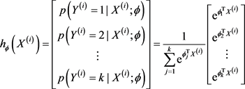(42)

where, denote model parameters vector, the cost function is as following:

(43)

where, denotes:

(44)

There are no closed form solutions to minimize the cost function Equation (43) at present. Therefore, we use the iterative optimization algorithm (for example, gradient descent method or L-BFGS). After derivation we get gradient formula is as following:

(45)

Then make the following update operation:

(46)

where, denotes learning rate.

3) Deep belief network embedded with Softmax regress (DBNESR)

DBN uses a Markov random field Restricted Boltzmann Machine (RBM) [52] [53] of unsupervised learning networks as building blocks for the multi-layer learning systems and uses a supervised learning algorithm named BP (back propagation) for fine-tuning after pre-training. Its architecture is shown in Figure 7. The deep architecture is a fully interconnected directed belief nets with one input layer, hidden layers, and one labeled layer at the top. The input layer has D units, equal to the number of features of samples. The label layer has C units, equal to the number of classes of label vector Y. The numbers of units for hidden layers, currently, are pre-defined according to the experience or intuition. The seeking of the mapping function, here, is transformed to the problem of finding the parameter space for the deep architecture [54].

The semi-supervised learning method based on DBN architecture can be divided into two stages: First, DBN architecture is constructed by greedy layer-wise unsupervised learning using RBM as building blocks. All samples are utilized to find the parameter space W with N layers. Second, DBN architecture is trained

Figure 7. Architecture of deep belief network embedded with Softmax regress (DBNESR).

according to the log-likelihood using gradient descent method. As it is difficult to optimize a deep architecture using supervised learning directly, the unsupervised learning stage can abstract the hierarchical representations feature effectively, and prevent over-fitting of the supervised training. The algorithm BP is used pass the error top-down for fine-tuning after pre-training.

For unsupervised learning, we define the energy of the joint configuration as [50]:

(47)

where, are the model parameters: is the symmetric interaction term between unit i in the layer and unit j in the layer,. is the ith bias of layer and is the jth bias of layer. is the number of units in the kth layer. The network assigns a probability to every possible data via this energy function. The probability of a training data can be raised by adjusting the weights and biases to lower the energy of that data and to raise the energy of similar, confabulated data that would prefer to the real data. When we input the value of, the network can learn the content of by minimizing this energy function.

The probability that the model assigns to a is:

(48)

(49)

where, denotes the normalizing constant. The conditional distributions over and are given as:

(50)

(51)

The probability of turning unit j is a logistic function of the states and:

(52)

The probability of turning unit i is a logistic function of the states of and:

(53)

where, the logistic function been chosen is the sigmoid function:

(54)

The derivative of the log-likelihood with respect to the model parameter can be obtained from Equation (48):

(55)

where, denotes an expectation with respect to the data distribution and denotes an expectation with respect to the distribution defined by the model [55]. The expectation cannot be computed analytically. In practice, is replaced by, which denotes a distribution of samples when the feature detectors are being driven by reconstructed. This is an approximation to the gradient of a different objective function, called the contrastive divergence (CD) [56] [57] [58] [59]. Using Kullback-Leibler distance to measure two probability distribution “diversity”, represented by, is shown in Equation (56):

(56)

where, denotes joint probability distribution of initial state of RBM network, denotes joint probability distribution of RBM network after n transformations of Markov chain Monte Carlo(MCMC), denotes joint probability distribution of RBM network at the ends of MCMC. Therefore, can be regarded as a measure location for between and. It constantly assigns to and gets new and. The experiments show that will tend to zero and the accuracy is approximate of MCMC after making slope for r times for correction parameter. The training process of RBM is shown in Figure 8.

We can get Equation (57) by training process of RBM using contrastive divergence:

(57)

where, is the learning rate. Then the parameter can be adjusted through:

(58)

where, is the momentum.

The above discussion is based on the training of the parameters between hidden layers with one sample x. For unsupervised learning, we construct the deep architecture using all samples by inputting them one by one from layer, train the parameters between and. Then is constructed, the value of is calculated by and the trained parameters between and. We also can use it to construct the next layer and so on. The deep architecture is constructed layer by layer from bottom to top. In each time, the parameter space is trained by the calculated data in the layer. Accord to the calculated above, the layer is obtained as below for a sample x fed from layer:

(59)

For supervised learning, the DBM architecture is trained by C labeled data. The optimization problem is formulized as:

Figure 8. Training process of RBM using contrastive divergence.

(60)

namely, to minimize cross-entropy. Where, denotes the real label probability and denotes the model label probability.

The greedy layer-wise unsupervised learning is just used to initialize the parameter of deep architecture, the parameters of the deep architecture are updated based on Equation (58). After initialization, real values are used in all the nodes of the deep architecture. We use gradient-descent through the whole deep architecture to retrain the weights for optimal classification.

6. Experiments

1) Face Recognition Databases

We selected some typical databases of images, for example ORL Face Database, which consists of 10 different images for each of the 40 distinct individuals. Each people is imaged in different facial expressions and facial details under varying lighting conditions at different times. All the pictures are captured with a dark background and the individuals are in an upright and frontal position; the facial gestures are not identical, expressions, position, angle and scale are some different; The depth rotation and plane rotary can be up to 20˚, the scale of faces also has as much as 10% change. For each face database as above, we randomly choose a part of images as training data and the remaining as testing data. In this paper, in order to reflect the universality and high efficiency of all classification algorithms we randomly choose about 50% of each individual image as training data and the rest as testing data. At first all images will be made preprocessing and feature extraction.

All the experiments are carried out in MATLAB R2010b environment running on a desktop with Intel^Ò Core^TM2 Duo CPU T6670 @2.20GHz and 4.00 GB RAM.

2) Relevant experiments

Experiment 1. In this experiment, we use median filtering to make smoothing denoising for images preprocessing and get the sample Figure 9 as following:

Seeing from the comparison of face images, the face images after filtering eliminate most of noise interference.

Experiment 2. In this experiment, we make histogram equalization for the images preprocessing and get the sample figures as following:

From Figure 10 and Figure 11 we can see: After histogram equalization, the distribution of image histogram is more uniform, the range of gray increases some and the contrast has also been stronger. In addition, the image after histogram equalization basically eliminated the influence of illumination, expanded the representation range of pixel gray, improved the contrast of image,

Figure 9. Face images with median filtering versus no median filtering.

Figure 10. Face images before histogram equalization versus after histogram equalization. (a) Original image; (b) Image after histogram equalization.

Figure 11. Histogram of original image versus histogram of image after histogram equalization. (a) Histogram of original image; (b) Histogram of image after histogram equalization.

made the facial features more evident and is conducive to follow-up feature extraction and FR.

Experiment 3. In this experiment, we employ multi-scale two-dimensional wavelet transform to generate the initial geometric features for representing face images. By the experiment we get the sample figures as following:

From Figure 12 we can see: Although for compression of images (or dimensionality-reduced), LL sub-graph information capacity has decreased some, but still has very high resolution and the energy of wavelet domain did not decrease a lot. LL sub-graph can be well made for the follow-up feature extraction.

Experiment 4. In this experiment, we extract features respectively with PCA and 2D-PCA and compare their effects as following:

From Figure 13 we can see that the first several principal components contribution rates extracted with 2D-PCA are higher than the first several principal components contribution rates extracted with PCA. From Figure 14 we can see when the principal components are extracted for 20, the principal component

Figure 12. Multi-scal two-dimensional wavelet transform.

Figure 13. Principal component energy figure. Abscissa: principal components; ordinate: energy value.

Figure 14. Principal component accumulation contribution rate. Abscissa: principal components; ordinate: total energy value.

contribution rate of 2D-PCA is greater than 90%, while the principal component contribution rate of PCA is less than 80%. Accordingly, 2D-PCA can use less principal component to better describe the image than PCA.

Figure 15 is the comparing results image of reconstruction with the feature respectively extracted with PCA and 2D-PCA. We can see that the images of reconstruction by 2D-PCA are clearer than the images of reconstruction by PCA when extracting same number of principal components. The reconstruction face extracted 50 principal components by 2D-PCA is almost same clear with the original image. 2D-PCA has better effect than PCA.

Experiment 5. In this experiment, we compare the recognition rate of the methods respectively based on PCA + BP, WT + PCA + BP, PCA + HBPNNs and WT + PCA + HBPNNs. The experiment is repeated many times and takes the average recognition rate. The experimental results are shown in Table 1.

As shown in Table 1, Recognition rates of HBPNNs are improved very greatly being compared to BP, in the same classifier (BP or HBPNNs) recognition rates of the methods based on WT + PCA are higher than them based on PCA.

Experiment 6. This experiment compares the recognition rate of the methods respectively based on WT + 2D-PCA + RBF and WT + 2D-PCA + HRBFNNs. The experiment is repeated for many times and takes the average recognition rate. The experimental results are shown in Table 2.

As shown in Table 2, Recognition rates of HRBFNNs are improved very greatly being compared to RBF. Therefore, HRBFNNs being used for FR is more feasible.

Experiment 7. Because SVM is essentially the classifier for two types, solving

Figure 15. Reconstructed images with 2D-PCA and PCA versus original image (t: principal component number). (a) Original image; (b) PCA principal component reconstruction images; (c) 2D-PCA principal component reconstruction images.

Table 1. Average recognition rates of different recognition methods.

Table 2. Average recognition rates of different recognition methods.

the multiple classification problems needs to reconstruct more appropriate classifier. We will use two methods of “One-Against-One” and “One-Against-the Rest” for the experiment and choose the method with better effect to construct the multiple classification classifiers of SVM. The experiment is repeated for 20 times and takes the average recognition rate. The experimental results are shown in Table 3.

As shown in Table 3, “One-Against-One” SVM has higher recognition rate than “One-Against-the-Rest” SVM and at the same time has lower wrong number. Therefore, we use the way of “One-Against-One” to reconstruct the SVM classifier to realize FR.

Experiment 8. In the paper we construct the multiple classification decision fusion classifier (MCDFC)—hybrid HBPNNs-HRBFNNs-SVM classifier. In this experiment, in order to show the efficiency of MCDFC, we first make recognition experiment respectively based on HBPNNs, HRBFNNs and SVM, then use the decision function to make fusions for classification results of three classifiers and get classification results of MCDFC. The experiment is repeated for 20 times and the experimental results are shown in Table 4 and in Figure 16.

As shown in Figure 16, the recognition effect of MCDFC is always not lower than the average level of other three kinds of classifiers and in almost all cases the effect of MCDFC is optimal.

To eliminate the error of single experiment and greatly reduce the random uncertainty, Table 5 lists the average recognition rates of each classifier for 20 times and the variance of each classifier. It can be seen from the experimental results that the multiple classification decision fusion classifier (MCDFC)—hybrid HBPNNs-HRBFNNs-SVM classifier has the best effect for FR, has the minimum variance, can effectively improve the generalization ability and has high stability.

Experiment 9. In this experiment, in order to validate the performance of our proposed algorithm—DBNESR is optimal for FR, we compare our proposed algorithm with some other methods such as BP, HBPNNs, RBF, HRBFNNs, SVM and MCDFC.

Table 3. Average recognition rates of different recognition methods.

Table 4. Recognition rates of different recognition methods for 20 times.

Table 5. Average recognition rates and variances of different recognition methods.

Figure 16. The curve figures of recognition rates of different recognition methods.

In the experiment we set up different hidden layers and each hidden layer with different neurons. The architecture of DBNESR is similar with DBN, but with a different loss function introduced for supervised learning stage. For greedy layer-wise unsupervised learning we train the weights of each layer independently with the different epochs, we also make fine-tuning supervised learning for the different epochs. All DBNESR structures and learning epochs used in this experiment are separately shown in Table 6. The number of units in input layer is the same as the feature dimensions of the dataset.

Almost all the recognition rates of these DBNESR structures are more than 90%, in particular the effects of the models of 500-1000-40 and 1000-500-40 are

Table 6. Different hidden layers of DBNESR and learning epochs used in this experiment.

Table 7. Recognition rates of different recognition methods for 20 times.

Table 8. Average recognition rates and variances of different recognition methods.

best and most stable. Therefore, the DBNESR structures used in this experiment are 1000-500-40, which represents the number of units in output layer is 40, and in 2 hidden layers are 1000 and 500 respectively. The learning rate is set to dynamic value, which the initial learning rate is set to 0.1 and becomes smaller as the training error becoming smaller. The experimental results are shown in Table 7, Table 8 and in Figures 17-19.

Figure 17. The curve figures of recognition rates of different recognition methods.

Figure 18. The bar charts of average recognition rate of different recognition methods.

Figure 19. The bar charts of variance of different recognition methods.

As shown in Table 7, Table 8 and in Figures 17-19, our proposed algorithm—DBNESR is optimal for FR, in almost all cases the recognition rates of DBNESR is highest and most stable, namely there is the largest average recognition rate and the smallest variance.

7. Conclusion

The conducted experiments validate that the proposed algorithm DBNESR is optimal for face recognition with the highest and most stable recognition rates, that is, it successfully implements hierarchical representations’ feature deep learning for face recognition. You can also be sure that it reflects hierarchical representations of feature by DBNESR in terms of its capability of modeling other artificial intelligent tasks, which is also what we’re going to do in the future.

Acknowledgements

This research was funded by the National Natural Science Foundation (Grand 61171141, 61573145), the Public Research and Capacity Building of Guangdong Province (Grand 2014B010104001), the Basic and Applied Basic Research of Guangdong Province (Grand 2015A030308018), the Main Project of the Natural Science Fund of Jiaying University (grant number 2017KJZ02) and the key research bases being jointly built by provinces and cities for humanities and social science of regular institutions of higher learning of Guangdong province (Grant number 18KYKT11), the cooperative education program of Ministry of Education (Grant number 201802153047), the college characteristic innovation project of Education Department of Guangdong province in 2019 (Grant number 2019KTSCX169), the authors are greatly thanks to these grants.

Compliance with Ethical Standards

1) (In Case of Funding) Funding

This study was funded by the National Natural Science Foundation (grant number 61171141, 61573145), the Public Research and Capacity Building of Guangdong Province (grant number 2014B010104001), the Basic and Applied Basic Research of Guangdong Province (grant number 2015A030308018), the Main Project of the Natural Science Fund of Jiaying University (grant number 2017KJZ02) and the key research bases being jointly built by provinces and cities for humanities and social science of regular institutions of higher learning of Guangdong province (grant number 18KYKT11), the cooperative education program of ministry of education (grant number 201802153047), the college characteristic innovation project of education department of guangdong province in 2019 (grant number 2019KTSCX169).

2) (If Articles Do Not Contain Studies with Human Participants or Animals by Any of The Authors, Please Select One of The Following Statements) Ethical Approval:

This article does not contain any studies with human participants or animals performed by any of the authors.

Conflicts of Interest

Hai-Jun Zhang declares that he has no conflict of interest. Ying-hui Chen declares that she has no conflict of interest.

References

[1]	Wright, J., Ma, Y., Mairal, J., et al. (2010) Sparse Representation for Computer Vision and Pattern Recognition. Proceedings of the IEEE, 98, 1031-1044. https://doi.org/10.1109/JPROC.2010.2044470
[2]	Wang, S.J., Yang, J., Sun, M.F., et al. (2012) Sparse Tensor Discriminant Color Space for Face Verification. IEEE Transactions on Neural Networks and Learning Systems, 23, 876-888. https://doi.org/10.1109/TNNLS.2012.2191620
[3]	Xu, Y., Zhong, A., Yang, J. and Zhang, D. (2010) LPP Solution Schemes for Use with Face Recognition. Pattern Recognition, 43, 4165-4176. https://doi.org/10.1016/j.patcog.2010.06.016
[4]	Fan, Z.Z., Xu, Y., Zuo, W.M., Yang, J., et al. (2014) Modified Principal Component Analysis: An Integration of Multiple Similarity Subspace Models. IEEE Transactions on Neural Networks and Learning Systems, 25, 1538-1552. https://doi.org/10.1109/TNNLS.2013.2294492
[5]	Yang, W.K., Sun, C.Y. and Zhang, L. (2011) A Multi-Manifold Discriminant Analysis Method for Image Feature Extraction. Pattern Recognition, 44, 1649-1657. https://doi.org/10.1016/j.patcog.2011.01.019
[6]	Xu, Y., Li, X., Yang, J., et al. (2013) Integrating Conventional and Inverse Representation for Face Recognition. IEEE Transactions on Cybernetics, 44, 1738-1746.
[7]	Wang, S.J., Zhou, C.G., Chen, Y.H., et al. (2011) A Novel Face Recognition Method Based on Sub-Pattern and Tensor. Neurocomputing, 74, 3553-3564. https://doi.org/10.1016/j.neucom.2011.06.017
[8]	Zhang, H.Z., Zhang, Z., Li, Z.M., Chen, Y. and Shi, J. (2014) Improving Representation Based Classification for Robust Face Recognition. Journal of Modern Optics, 61, 961-968. https://doi.org/10.1080/09500340.2014.915064
[9]	Wang, S.J., Chen, H.L., et al. (2014) Face Recognition and Micro-Expression Recognition Based on Discriminant Tensor Subspace Analysis Plus Extreme Learning Machine. Neural Processing Letters, 39, 25-43. https://doi.org/10.1007/s11063-013-9288-7
[10]	Wan, W.G., Zhou, Z.H., Zhao, J.W. and Cao, F.L. (2015) A Novel Face Recognition Method: Using Random Weight Networks and Quasi-Singular Value Decomposition. Neurocomputing, 151, 1180-1186. https://doi.org/10.1016/j.neucom.2014.06.081
[11]	Zhao, Z. and Liu, H. (2007) Spectral Feature Selection for Supervised and Unsupervised Learning. Proceedings of the 24th International Conference on Machine Learning, Corvails, June 2007, 1151-1157. https://doi.org/10.1145/1273496.1273641
[12]	Cai, D., Zhang, C.Y. and He, X.F. (2010) Unsupervised Feature Selection for Multi-Cluster Data. Proceedings of the 16th SIGKDD International Conference on Knowledge Discovery and Data Mining, July 2010, Washington DC, 333-342. https://doi.org/10.1145/1835804.1835848
[13]	Zhao, Z., Wang, L. and Liu, H. (2010) Efficient Spectral Feature Selection with Minimum Redundancy. Proceedings of the 24th AAAI Conference on Artificial Intelligence, July 2010, Atlanta, 673-678.
[14]	Hou, C.P., Nie, F.P. and Li, X.L. (2011) Joint Embedding Learning and Sparse Regression: A Framework for Unsupervised Feature Selection. IEEE Transactions on Cybernetics, 44, 793-804.
[15]	Ghazali, K.H., Mansor, M.F. and Mustafa, M.M. (2007) A Feature Extraction Technique Using Discrete Wavelet Transform for Image Classification. Proceedings of the 5th Student Conference on Research and Development, Selangor, Malaysia, 12-11 December 2007, 1-4. https://doi.org/10.1109/SCORED.2007.4451366
[16]	Hu, H.F. (2011) Variable Lighting Face Recognition Using Discrete Wavelet Transform. Pattern Recognition Letters, 32, 1526-1534. https://doi.org/10.1016/j.patrec.2011.06.009
[17]	Jemai, O., Zaied, M., Amar, C.B. and Alimi, A.M. (2010) FBWN: An Architecture of Fast Beta Wavelet Networks for Image Classification. Proceedings of the 2010 International Joint Conference on Neural Networks (IJCNN), Barcelona, 18-23 July 2010, 1-8. https://doi.org/10.1109/IJCNN.2010.5596876
[18]	Huang, K. and Aviyente, S. (2008) Wavelet Feature Selection for Image Classification. IEEE Transactions on Image Processing, 17, 1709-1719. https://doi.org/10.1109/TIP.2008.2001050
[19]	Zhao, M., Li, P. and Liu, Z. (2008) Face Recognition Based on Wavelet Transform Weighted Modular PCA. 2008 Congress on Image and Signal Processing, Sanya, 27-30 May 2008, 589-593. https://doi.org/10.1109/CISP.2008.138
[20]	Zhang, B.L., Zhang, H.H. and Ge, S.S. (2004) Face Recognition by Applying Wavelet Subband Representation and Kernel Associative Memory. IEEE Transactions on Neural Networks, 15, 166-177. https://doi.org/10.1109/TNN.2003.820673
[21]	Nefian A.V., Hayes, M.H. (1998) Face Detection and Recognition Using Hidden Markov Models. Proceedings 1998 International Conference on Image Processing, ICIP98 (Cat. No. 98CB36269), Chicago, 7-7 October 1998, 141-145. https://doi.org/10.1109/ICIP.1998.723445
[22]	Vlasenko, B., Prylipko, D., Böck, R. and Wendemuth, A. (2013) Modeling Phonetic Pattern Variability in Favor of the Creation of Robust Emotion Classifiers for Real-Life Applications. Computer Speech & Language, 28, 483-500. https://doi.org/10.1016/j.csl.2012.11.003
[23]	He, L., Lech, M., Maddage, N.C. and Allen, N.B. (2011) Study of Empirical Mode Decomposition and Spectral Analysis for Stress and Emotion Classification in Natural Speech. Biomedical Signal Processing and Control, 6, 139-146. https://doi.org/10.1016/j.bspc.2010.11.001
[24]	Suykens, J.A.K. and Vandewalle, J. (1999) Least Squares Support Vector Machine Classifiers. Neural Processing Letters, 9, 293-300. https://doi.org/10.1023/A:1018628609742
[25]	Lee, C.-C., Mower, E., Busso, C., Lee, S. and Narayanan, S. (2011) Emotion Recognition Using a Hierarchical Binary Decision Tree Approach. Speech Communication, 53, 1162-1171. https://doi.org/10.1016/j.specom.2011.06.004
[26]	Igelnik, B. and Pao, Y.H. (1995) Stochastic Choice of Basis Functions in Adaptive Function Approximation and the Functional-Link Net. IEEE Transactions on Neural Networks, 6, 1320-1329. https://doi.org/10.1109/72.471375
[27]	Pao, Y.H., Park, G.H. and Sobajic, D.J. (1994) Learning and Generalization Characteristics of the Random Vector Functional-Link Net. Neurocomputing, 6, 163-180. https://doi.org/10.1016/0925-2312(94)90053-1
[28]	Xu, Y., Zhang, X.F. and Gai, H.C. (2011) Quantum Neural Networks for Face Recognition Classifier. Procedia Engineering, 15, 1319-1323. https://doi.org/10.1016/j.proeng.2011.08.244
[29]	Reddy, K.R.L., Babu, G.R. and Kishore, L. (2010) Face Recognition Based on Eigen Features of Multi Scaled Face Components and an Artificial Neural Network. Procedia Computer Science, 2, 62-74. https://doi.org/10.1016/j.procs.2010.11.009
[30]	Suka, H.-I., Lee, S.-W., Shen, D.G. and the Alzheimer’s Disease Neuroimaging Initiative (2014) Hierarchical Feature Representation and Multimodal Fusion with Deep Learning for AD/MCI Diagnosis. Neuroimage, 101, 569-582. https://doi.org/10.1016/j.neuroimage.2014.06.077
[31]	Han, H., Shan, S.G., Chen, X.L. and Gao, W. (2013) A Comparative Study on Illumination Preprocessing in Face Recognition. Pattern Recognition, 46, 1691-1699. https://doi.org/10.1016/j.patcog.2012.11.022
[32]	Chao, S. (2013) Research and Implement of Face Recognition Based on Neural Network. South China University of Technology, Guangzhou.
[33]	Längkvist, M., Karlsson, L. and Loutfi, A. (2014) A Review of Unsupervised Feature Learning and Deep Learning for Time-Series Modeling. Pattern Recognition Letters, 42, 11-24. https://doi.org/10.1016/j.patrec.2014.01.008
[34]	Xu, Y.J., You, T. and Du, C.L. (2015) An Integrated Micromechanical Model and Bp Neural Network for Predicting Elastic Modulus of 3-D Multi-Phase and Multi-Layer Braided Composite. Composite Structures, 122, 308-315. https://doi.org/10.1016/j.compstruct.2014.11.052
[35]	Andrew, N. and Ngiam, J., et al. (2014) http://ufldl.stanford.edu/wiki/index.php/Backpropagation_Algorithm
[36]	Zhang, Y.X., Gao, X.D. and Katayama, S. (2015) Weld Appearance Prediction with BP Neural Network Improved by Genetic Algorithm during Disk Laser Welding. Journal of Manufacturing Systems, 34, 53-59. https://doi.org/10.1016/j.jmsy.2014.10.005
[37]	Sundararajan, N. and Saratchandran, P. (1998) Parallel Architecture for Artificial Neural Networks: Paradigms and Implementations. IEEE Computer Society Press, 412.
[38]	Han, L.Q. (2007) Artificial Neural Networks Tutorial. Beijing University of Posts and Telecommunications Press of China, Beijing, 47-83.
[39]	Karami, A. and Guerrero-Zapata, M. (2015) A Hybrid Multiobjective RBF-PSO Method for Mitigating DoS Attacks in Named Data Networking, Neurocomputing, 151, 1262-1282. https://doi.org/10.1016/j.neucom.2014.11.003
[40]	Reiner, P. and Wilamowski, B.M. (2015) Efficient Incremental Construction of RBF Networks Using Quasi-Gradient Method. Neurocomputing, 150, 349-356. https://doi.org/10.1016/j.neucom.2014.05.082
[41]	Liu, X.F., Bo, L. and Luo, H.L. (2015) Bearing Faults Diagnostics Based on Hybrid LS-SVM and EMD Method. Measurement, 59, 145-166. https://doi.org/10.1016/j.measurement.2014.09.037
[42]	Wang, Z.G., Zhao, Z.S., Weng, S.F. and Zhang, C.S. (2015) Solving One-Class Problem with Outlier Examples by SVM. Neurocomputing, 149,100-105. https://doi.org/10.1016/j.neucom.2014.03.072
[43]	Al-Hadeethi, H., Abdulla, S., Diykh, M., Deo, R.C. and Green, J.H. (2020) Adaptive Boost LS-SVM Classification Approach for Time-Series Signal Classification in Epileptic Seizure Diagnosis Applications. Expert Systems with Applications, 161, Article ID 113676. https://doi.org/10.1016/j.eswa.2020.113676
[44]	Yin, H.P., Jiao, X.G., Chai, Y. and Fang, B. (2015) Scene Classification Based on Single-Layer SAE and SVM. Expert Systems with Applications, 42, 3368-3380. https://doi.org/10.1016/j.eswa.2014.11.069
[45]	Liu, X.F. and Bo, L. (2015) Identification of Resonance States of Rotor-Bearing System Using RQA and Optimal Binary Tree SVM. Neurocomputing, 152, 36-44. https://doi.org/10.1016/j.neucom.2014.11.021
[46]	Dasgupta, S. and Ng, V. (2009) Mine the Easy, Classify the Hard: A Semi-Supervised Approach to Automatic Sentiment Classification. Proceedings of the Joint Conference of the 47th Annual Meeting of the Association for Computational Linguistics and 4th International Joint Conference on Natural Language Processing of the AFNLP, Suntec, Singapore, August 2009, 701-709. https://doi.org/10.3115/1690219.1690244
[47]	Zhu, X. (2007) Semi-Supervised Learning Literature Survey. Technical Report, University of Wisconsin Madison, Madison.
[48]	Schmidhuber, J. (2015) Deep Learning in Neural Networks: An Overview. Neural Networks, 61, 85-117. https://doi.org/10.1016/j.neunet.2014.09.003
[49]	Bengio, Y. (2007) Learning Deep Architectures for AI. Technical Report, IRO, Universite de Montreal, Montreal.
[50]	Hinton, G.E. and Salakhutdinov, R. (2006) Reducing the Dimensionality of Data with Neural Networks. Science, 31, 3504-3507. https://doi.org/10.1126/science.1127647
[51]	Hu, W.P., Qian, Y., Soong, F.K. and Wang, Y. (2015) Improved Mispronunciation Detection with Deep Neural Network Trained Acoustic Models and Transfer Learning Based Logistic Regression Classifiers. Speech Communication, 67, 154-166. https://doi.org/10.1016/j.specom.2014.12.008
[52]	Fischera, A. and Igelb, C. (2014) Training Restricted Boltzmann Machines: An Introduction. Pattern Recognition, 47, 25-39. https://doi.org/10.1016/j.patcog.2013.05.025
[53]	Lopes, N. and Ribeiro, B. (2014) Towards Adaptive Learning with Improved Convergence of Deep Belief Networks on Graphics Processing Units. Pattern Recognition, 47, 114-127. https://doi.org/10.1016/j.patcog.2013.06.029
[54]	Zhou, S.S., Chen, Q.C. and Wang, X.L. (2014) Fuzzy Deep Belief Networks for Semi-Supervised Sentiment Classification. Neurocomputing, 131, 312-322. https://doi.org/10.1016/j.neucom.2013.10.011
[55]	Salakhutdinov, R. and Murray, I. (2008) On the Quantitative Analysis of Deep Belief Networks. Proceedings of the 25th International Conference on Machine Learning, Helsinki, Finland, August 2008, 872-879. https://doi.org/10.1145/1390156.1390266
[56]	Hinton, G.E. (2002) Training Products of Experts by Minimizing Contrastive Divergence. Neural Computation, 14, 1771-1800. https://doi.org/10.1162/089976602760128018
[57]	Zhang, H.-J., Zhang, N. and Xiao, N.-F. (2015) Fire Detection and Identification Method Based on Visual Attention Mechanism. Optik, 126, 5011-5018. https://doi.org/10.1016/j.ijleo.2015.09.167
[58]	Zhang, H.-J. and Xiao, N.-F. (2016) Parallel Implementation of Multilayered Neural Networks Based on Map-Reduce on Cloud Computing Clusters. Soft Computing, 20, 1471-1483. https://doi.org/10.1007/s00500-015-1599-3
[59]	Zhang, H.-J. and Xiao, N.-F. (2015) Learning Hierarchical Representations for Face Recognition Using Deep Belief Network Embedded with Softmax Regress and Multiple Neural Networks. Proceedings of the 2015 2nd International Workshop on Materials Engineering and Computer Sciences (IWMECS), 1-7 https://doi.org/10.2991/iwmecs-15.2015.1