Development and Parallelization of an Improved 2D Moving Window Standard Deviation Python Routine for Image Segmentation Purposes ()
1. Introduction
Image segmentation consists of partitioning image pixels into a set of regional categories [1] [2]. This process can be significantly improved by using two additional images (image features) based on two fundamental statistical concepts, if they are also input to neural networks [2], a technique that creates a fertile field for segmentation solutions [3] [4] [5] [6]. These image features can be seen in Figure 1 and are described as follows:
1) n × n moving window average (MWA): classical MWA, where the value of the central pixel in the array is replaced by its n × n window average; and
1) n × n moving window standard deviation (MWSD): similar to the MWA, but the value of the central pixel is replaced by the standard deviation of the moving array.
Local window functions are not restricted to image segmentation: they are routinely used for suppressing noise in filter operations [7] [8]. That aside, their usage in segmentation is well established in the literature [2] [9] [10].
The first image attribute (MWA) is calculated by convolving the original image with a specific kernel, which is a matrix filled by 1/n2. Furthermore, these convolutions can be calculated in a faster way via products in a frequency domain. Likewise, this process can get even faster by integrating a method called “overlap-and-add”. In this case, if the inputs are N × N arrays, the computational time is given by O(N2 log2n) [11], which is much lesser than a naïve convolution algorithm’s: O(N2 n2).
Any process that can be written in convolutional terms (as MWA) can be implemented in such a way to get these benefits. However, the MWSD has a restriction, since the standard deviation is not a linear operation itself, and has the same computational complexity as a naïve convolution algorithm (O(N2 n2)).
As the square dependency with N cannot be solved in any of the mentioned algorithms, the important variable to pay attention here is n: the moving window side length.
Choosing useful n × n kernel dimensions for a specific process is usually made as a heuristic trial and error process, and depends on the data properties, especially spatial resolution and noise signature. The growth of SAR spatial resolution in the last decades comes with downside of bigger image dimensions. At the same proportion, the kernel window size search space is increased. As an example, a 3 × 3 MWA applied over an old ENVISAT ASAR sensor data would get similar results to applying a 45 × 45 MWA over new Sentinel-1 data, in spatial terms, while in this last case the equivalent computation would be 225 times slower.
Therefore, the core of this article is to propose a new methodology using an algorithm that replaces the usual 2D MWSD, in order to decrease its computational complexity, as there are no other works dealing with this problem and a researcher needs freedom to study various kernel sizes in a timely manner in
![]()
Figure 1. Original Sentinel-1 image and two image features.
order to find the one that best fits his models. The idea behind it is saving some of the calculations done at the first pixel of a row to the next one and so on, after an optimized analytical reformulation of the standard deviation calculation is performed. Additionally, our algorithms were thought to be used in context of CPU parallelism, being intelligently designed to take advantage with a faster runtime.
Following strong open source global trends, and seeking to benefit the maximum of users, our codes were written in Python, as this language is commonly used in the context of machine learning, and is available online in a public GitHub repository.
Python is indeed developed to be a high-level, interpreted language and as consequence, generally slower than C or Fortran at runtime [12], but this problem is already addressed by free packages that allow python compilation and lower level optimization of code.
The Numba package [13] is an example. Described as “a high-performance Python compiler”, Numba is a Python library meant to compile Python functions (even though it is an interpreted language by default). By doing this, they gain C-like velocity, being generally compatible with NumPy—a widely used linear algebra package for Python.
This work was developed as part of a set of digital image processing routines, to be an improved tool for automatic classifiers already used in remote sensing studies, which aims to make a comparison between the usual performance of the 2D MWSD algorithm and ours, before and after being compiled with Numba.
2. Methodology
First, the methodological process was developed with three test algorithms: 1) a “didactic” MWSD, 2) a “better” MWSD and 3) an “optimized” MWSD. These algorithms are introduced and discussed below for a 1D matrix and a 1D window. After the first theoretical assessments stage, the first and last algorithms were extended to the second dimension (2D input array and 2D window). They were programmed and tested both theoretically and practically, before and after being compiled, so that we can compare them in terms of computational efficiency.
2.1. Didactic Algorithm
For didactic purposes, the standard deviation of a series of observations is defined in terms of its variance—an average over all squared differences between the observations and their average value—as in Equation (1):
, (1)
where σ is the standard deviation of ne elements xi, and
is their mean value. The standard deviation of a dataset serves as a measure of how disperse are its elements. As
is part of the calculation, this process takes a total of 4ne + 1 operations.
The denominator ne is sometimes exchanged with ne − 1, what is called Bessel’s correction [14] [15] and is useful to remove part of standard deviation estimator bias when ne is small. We are not going to use Bessel’s correction in this article, as it is not relevant for image segmentation.
From a generic 1D array of N elements, it’s possible to create another of similar shape, so that each element i therein is the standard deviation of 3 adjacent values in the original array, making a window centered at the ith position. When one of the values does not exist in these windows, we make it zero for the sake of calculation. This array is the result of a one-dimensional MWSD over the original array.
This process is equivalent to pad the older array with zeros, then slide a window of size, n = 3, through that array, method already proposed in the literature [16]. Every time the window is updated, a standard deviation is calculated, and the result stacked in the new array. This process takes then 13N operations, or in a more general case, for any window size n, N(4n + 1).
This method is effective. However, in many cases, it has an extense processing time. There are many faster ways to calculate MWSD, and an example is shown in next section.
2.2. Better Algorithm
In order to develop a more efficient algorithm, simple manipulation of Equation (1) can lead to Equation (2):
(2)
With no more tricks, this formula makes computing the standard deviation of an array of n e elements much faster: only 3ne + 3 operations are needed, as one only loop must be used. Also, thinking about the problem just exposed in last section about 1D MWSD calculation, we would only make N(3n + 3) operations to get the same task done. In other words, when the window size, n, gets big, approximately 1/4 less operations are made. It’s important to observe that efficiency and intelligibility do not go hand in hand: Equation (2) would not be a good introduction formula to standard deviation.
2.3. Optimized Algorithm
Taking 1D MWSD is a problem that gets simplified if one takes a careful look on how variables are used in Equation (2). Note that if summations are not calculated from scratch at each array element, but instead just updated when the window moves, a python pseudo-code like “optimized_mwsd_1D” (in Code 1) would be gotten.
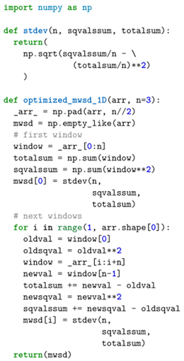
Code 1. Optimized 1D MWSD.
And here is the advantage: what we had previously gotten with N(3n + 3) operations now costs only 11N + 3n − 7 operations. When the array side (N) is sufficiently big, the task complexity does not depend on the chosen window side, n. As this number is usually an odd number greater or equal to 3—as the window used is centered at a certain position, from the stated problem, it is right to say that our new algorithm always performs faster than our previous one.
2.4. 2D Extension
When working with 2D input data arrays of N lines and M columns, it might be useful to extend the concept of a moving window standard deviation algorithm, in a way that a window represents a 2D array, and it will move through all the array points, being once centered at each one of them. In this way, n could now be a measure to the side of the window used.
Making such alterations to the didactic algorithm explained in section 2.1, would give us a simple algorithm that needs NM(4n2 + 1) operations to be run. It means that the computational time used for making these calculations would sensibly depend on the window size used. As N and M are usually big numbers in satellite remote sensing applications, this formula might be a problem.
As the optimized algorithm could make MWSD almost does not depend on n when N is sufficiently big, the same logic was tried to be applied at the new 2D case. What is essential about this code is that the algorithm behind it would do exactly what our previous done, but only making use of N(M(6n + 5) + 3n2 − 6n − 2) + 1: most part of the calculation is done by just updating (in the term 6NMn).
These numbers may be easily understood if we assume M
N n ≥ 3. In such case, the exposed formulas can be approximated to 4N2n2 and 6N2n, respectively. The latest algorithm performs faster than the first, even in the limit case, when n = 3. Another great advantage of this 2D algorithm is that, as it is basically running the extended 1D algorithm at each row, we can then parallelize loops over every column, as they only depend on previous operations therein.
There are many methods to parallelize Python code, for example: using Numba [13], Cython [17], and mpi4py [18]. As Python’s differential is that it conquers big results with little typing effort, Numba was chosen. It can frequently get almost perfect results by just changing a couple lines of code.
While Python is usually slow for calculations because it is an interpreted language, Numba is a Python library able to compile its codes, so that it runs in C-like velocity.
Getting started to Numba is a simple task. Compiling code with parallel support usually means importing the library and adding a decorator (a statement starting with @) one line before a Python function. An example is served in Code 2.
This decorator is a “just in time” compiler. It means it compiles the code when the function is first called. Although parallel argument is set to True, it just means that parallel support is enabled at compilation time. To actually make use of parallelization in our code we would need to go to the columns’ loop of our algorithm, and, instead of writing a regular range, use numba.prange for a parallel range iterator.
There is just another thing needed to be done: we previously used a function to pad the input array: “np.pad”. This function comes from NumPy library and has no compatibility with Numba. A simple function was developed to pad an array with zeros in order to finish the compilation process. There is a list of NumPy supported features in Numba’s official documentation, and it might be useful when debugging compilation.
3. Results and Discussion
The algorithms developed for preparing results bellow are publicly available online at github.com/marcosrdac/mwsd. Theoretical efficiency results for 1D and 2D MWSD problems can be seen in Figure 2. Algorithms’ complexities were described in Table 1. Real results can be seen in Figure 3. Each point was calculated five times, and error bars were plotted using standard deviation (with Bessel’s correction) as dispersion estimator.
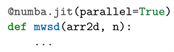
Code 2. @numba.jit decorator usage.
![]()
Table 1. Algorithms and their complexities.
![]()
Figure 2. Theoretical performance (in operations) vs. n plot for 1D and 2D algorithms (indicated by different line styles) and different values of N (indicated by different line colors).
![]()
Figure 3. Real performance (in time) vs. n plot for 2D algorithms (indicated by different line styles) and different values of N (indicated by different line colors).
It is useful to know that an MWSD algorithm made with Numpy’s “std” (the standard way a Python user would calculate standard deviation) function behaved just like “didactic” algorithm in terms of computational time.
Our results were plotted in log-log plots, so that the reader can explore how the number of operations scales with respect to n, in orders of magnitude. Different line colors mean curves made with different values of array side, N. On the other hand, the different line styles distinguish curves by the algorithm used. The established conventions for colors were:
· Red line: N = 100;
· Green line: N = 200;
· Orange line: N = 300; and
· Blue line: N = 400.
Also, these were the line style conventions:
· dotted line: means curve was calculated using didactic MWSD;
· dashed line: means curve was calculated using better MWSD;
· and continuous line: means curve was calculated using optimized MWSD.
The 1D optimized algorithm’s theoretical performance can be seen as the continuous lines at the first plot in Figure 2, and is visually almost independent from n, as expected. For n = 29, it does the same job than usual didactic 1D MWSD in an amount of time one order of magnitude bellow (compare continuous and dotted lines of the same colors).
The theoretical results get yet more interesting when talking about 2D algorithms (second plot of Figure 2). Our new algorithm is indeed faster than usual 2D MWSD, while performing the same accuracy. For a 19 pixels side window, these algorithms’ performance differs by one order of magnitude in time, and almost two of them, when window size gets to 59. Also, it’s important to know that, for greater values of N (or bigger array sizes), this difference gets even higher.
Real tests were only made for 2D algorithms, as they are useful for image segmentation. Their results were plotted in Figure 3. The first plot is a pure Python/NumPy code and could only be calculated for a small range of n’s: 3, 5, 7 and 9 as they were too time consuming. The time magnitude order is in seconds, and this happens because how non-compiled Python loops are highly inefficient. Although spent times do scale with n, this variation is not big enough when compared to the intrinsic slowness of python in the case of a small window and array sides. Our results show that the proposed algorithm (continuous line) consumes less computation time than the didactic MWSD even before compilation.
Some important effects are heavily seen in the bottom plot of Figure 3. The fundamental reason for them is that most part of the data stands near to the end of the plot, in consequence of the log-log plotting choice. It means that the curve trend must be visually estimated from there. Moreover, it’s known from basic calculus that polynomial curves are dominated by their term of highest exponent; the other terms’ effect is not important when abscissa get big [19]. In a log-log plot, different exponent terms are viewed as different line slopes. Based on that, the bottom plot of Figure 3 is remarkably similar to the expected plot in Figure 2’s right: the ending slopes of all curves are both visually and numerically tending to equality when n increases. It means that both didactic and optimized MWSD algorithms have the computational complexity that was previously expected in theory.
The difference between the behavior of these two plots is better visible at the first three points of the curves (n ≤ 9), and is completely understandable: theoretical formulas only account for MWSD, not for the previous process of padding the input array (that only exists to assert input and output arrays are of the same sizes) and allocating memory for output. This consumes a significant time for slow values of n and can be seen as a different, lesser slope at the beginning of the second plot of Figure 3. Besides this effect, its resemblance to the second plot of Figure 2 is clear and validates this article. We emphasize here the importance of computational time to the compiled algorithms’; their magnitude is in ms.
This technique is very useful in satellite remote sensing studies, as it can estimate textural characteristics of an image, being convenient to robust methods of segmentation, such as neural networks. As an example, oil slicks are easily seen in RADAR images. In number, “Interferometric Wide Single Look Complex” images are arrays of enormous dimensions, such as 13,169 × 17,241 px2. Applying this process to an 8192 × 8192 px2 subset using a didactic algorithm and n = 5 took 25 minutes to complete the process using four cores of an Intel i9 processor. After Numba compilation, this processing time went down to 11 seconds. Using our method we only needed 0.7 seconds to perform the same job. Therefore, if five images are needed to be processed by an MWSD algorithm, our method would run it in 45 seconds instead of the 12 minutes of the didactic algorithm, or 28 hours with the same algorithm without the Numba compilation.
4. Conclusions
In this paper, we demonstrated that moving window standard deviation functions can have their efficiency improved with two simple steps: 1) useful reformulation of analytic formula at the cost of losing certain amount of intuitive intelligibility and 2) reusing previous calculations in future iterations.
Our “optimized” (both 1D and 2D) code ran significantly faster than a naïve, completely “didactic” one, or even another that would be made using default NumPy functions. Pure Python is indeed very slow when evaluating loops and numerical results, as could be seen at our results, but this was solved by using Numba, with compilation and parallelization of code.
Image segmentation is useful in many areas but is of core knowledge when it comes to environmental control. Defining areas of significant atmospheric pollution, urban occupation levels, geologic faults, and ocean phenomena are key examples of its utilities. The proposed improvement is especially useful when working with satellite data, where images compose arrays of large dimensions, and even auxiliary processes can frequently take considerable amount of time.
Once our algorithm has a linear time dependency with the window side used, scientists can now feel free to study a higher variety spatial window sizes in order to produce their best models.
Future developments and implementations of this piece of code will be added to our investigations to study machine learning pixelwise segmentation of oil spills in satellite data.
Although MWA and MWSD were the only local window functions studied here, many other textural descriptors such as fractal dimension and entropy would be useful in window functions if more efficiently implemented. New works can also rethink this article achievement in a GPU parallelism perspective, as it grows to become a standard technique in high performance computing.
Acknowledgements
We are grateful to the Satellite Oceanography Laboratory (LOS) of the Geo-sciences Institute (IGEO) of the Federal University of Bahia (UFBA) for providing the facilities for the conduction of the experiments and data analysis. LOS is partially financially supported by the National Council for Scientific and Technological Development (CNPq—Research Grant #424495/2018-0). The first author also would like to thank the Undergraduate Research Mentorship Program at UFBA for his scholarship under the same research grant.