1. Introduction
Let  be independent observations of a
  valued random vector (X, Y) with
 . We estimate the regression function
  by the following form of kernel estimates
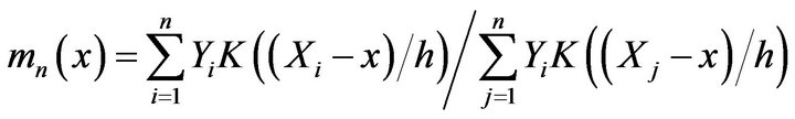 (1.1)
(1.1)
where  is called the bandwidth and K is a given nonnegative Borel kernel. The estimator (1.1) was first introduced by Nadaraya ([1]) and Watson ([2]). The studies of
  can also refer to, for examples, Stone ([3]), Schuster and Yakowitz ([4]), Gasser and Muller ([5]), Mack and Müller ([6]), Greblicki and Pawlak ([7]), Kohler, Krzyżak and Walk ([8,9]), and Walk ([10]). When point x is near the boundary of their support, the kernel regression estimator (1.1) has suffered from a serious problem of boundary effects. Hereafter 0/0 is treated as 0. For the kernel function we assume that
 (1.2)
(1.2)
and
 (1.3)
(1.3)
where ,
,  and
and  are positive constants,
  is either always
  or always
  norm,
norm,  denotes the indicator function of a set, and H is a bounded decreasing Borel function in
  such that
 (1.4)
(1.4)
Through this paper we assume that
 (1.5)
(1.5)
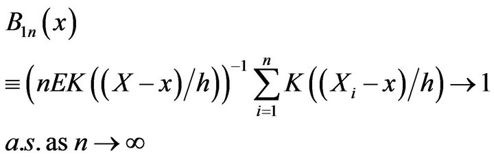
One of the fundamental problems of asymptotic study on nonparametric regression is to find the conditions under which  is a strongly consistent estimate of
  for almost all
  (µ probability distribution of X). The first general result in this direction belongs to Devroye ([11]), who established strong pointwise consistency of
  for bounded Y. Zhao and Fang ([12]) establish its strong consistency under the weaker condition that
  for some
 . However, the dominating function
  of (1.3) in the above literature is confined as
  for some
 . GreblickiKrzyżak and Pawlak ([13]) establish the complete convergence of
  for bounded Y and rather general dominating function H of (1.3) for almost all
 . This permits to apply kernels with unbounded support and even not integrable ones. In this paper, we establish the strong consistency of
  under the conditions of GKP ([13]) on the kernel and various moment conditions on Y, which provides a general approach for constructing strongly consistent kernel estimates of regression functions. We have Theorem 1.1 Assume that
  for some
 , and (1.2)-(1.5) are satisfied, and that
 (1.6)
(1.6)
Then
 (1.7)
(1.7)
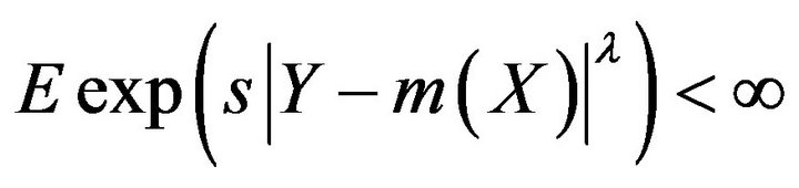
Theorem 1.2 Assume that  for some
  and
and , and (1.2)-(1.5) are met, and that
 (1.8)
(1.8)
Then (1.7) is true.
It is worthwhile to point out that in the above theorems we do not impose any restriction on the probability distribution µ of X.
2. Proof of the Theorems
For simplicity, denote by c a positive constant, by  a positive constant depending on x. These constants may assume different values in different places, even within the same expression. We denote by
  as a sphere of the radius r centered at x,
 .
.
Lemma 2.1 Assume that . For all
 there exists a nonnegative function
  with
with  such that for almost all
 ,
,
Refer to Devroye ([11]).
Lemma 2.2 Assume that (1.2)-(1.5) are satisfied. Let  be
be  integrable for some
 . Then

as  for almost all
 .
.
It is easily proved by using Lemma 1 of GKP ([13]).
Lemma 2.3 Assume that (1.2)-(1.5) are met, and that
 .
.
Then for almost all
Refer to GKP ([13]).
Now we are in a position to prove Theorems 1.1 and 1.2.
Proof. For simplicity, we write “for a.e. x” instead of the longer phrase “for almost all ”. Write

Since

and by Lemma 2.3, a.s. for a.e. x, it suffices to vertify that
  a.s. for a.e. x, or, to prove
  a.s. and
  a.s. for a.e. x.
Since  is convex in y for
 , and for fixed
  and
and ,
,  is convex in
 for large a, it follows from Jensen’s inequality that
  and
and 
when , and that
 and
and
 for some
  and
and 
when .
.
Write ,
,  (in Theorem 1.1) or
  (in Theorem 1.2). It follows that

and

by Borel-Cantelli’s lemma, and
 a.s. (2.1)
Write , if
, if . By (1.6) or
(1.8),  , we can take
  such that
 (2.2)
(2.2)
Put


By (1.3) and Lemma 2.1, for a.e. x,
 (2.3)
(2.3)
By Lemma 2.3,
 (2.4)
(2.4)
By Schwarz’s inequality, (2.1), (2.3) and (2.4),
 (2.5)
(2.5)
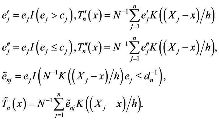
Write
We have  Take
Take
 . Since
  for
for , we have
and

By Lemma 2.2,
 .
.
By (2.2) and (2.3),

Given , it follows that for a.e. x and for n large,
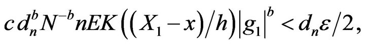 (2.6)
(2.6)
and

By Borel-Cantelli’s lemma and for a.e. x,
 for any
 we have
 a.s for a.e. x Since, by Lemma 2.2, for a.e. x

we have
 a.s for a.e. x, as
 . (2.7)
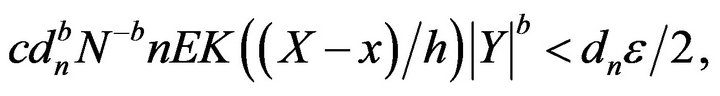
By (2.2) and (2.3), when , for a.e. x,

and for n large,  and
and
 a.s. for a.e. x. (2.8)
By (2.5) and (2.8), noticing that  , we have
 a.s for a.e. x. (2.9)
To prove  a.s for a.e. x, we write
  , and put
By using the same argument as above,
 a.s.
a.s.
and for a.e. x,
 (2.10)
Also, for a.e. x and for n large,
 and
and  (2.11)
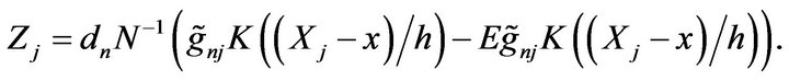
Write , then
 . Take
 . Since
 for
for , we have

and

By Lemma 2.2, for a.e. x,

Given , similar to (2.6), for a.e. x and n large,
 and
and

and it follows that
 a.s. for a.e. x (2.12)
from
 for a.e. x and
and Borel-Cantelli’s lemma.
By (2.10)-(2.12),
 a.s. for a.e. x and
 a.s. for a.e. x (2.13)
Replacing  by
by , it implies that
 a.s. for a.e. x (2.14)
(2.13) and (2.14) give
 a.s. for a.e. x (2.15)
The theorems follow from (2.9) and (2.15).
3. Acknowledgements
Cui’s research was supported by the Natural Science Foundation of Anhui Province (Grant No.1308085MA02), the National Natural Science Foundation of China (Grant No. 10971210), and the Knowledge Innovation Program of Chinese Academy of Sciences (KJCX3-SYW-S02).